KANDA DATA

Residual values play an important role in linear regression analysis. These residuals are used for OLS assumption tests, such as normality tests and heteroskedasticity tests. For instance, one of the key assumptions in linear regression analysis is that the residuals are normally distributed.

Therefore, we need to first calculate the residual values before proceeding with a normality test. In this article, Kanda Data will provide a tutorial on how to easily obtain residual values using Excel. Specifically, we will explain how to automatically display residual values during regression analysis in Excel.

Definition of Residuals

Before continuing with the tutorial, it is important to first understand what residuals are. A residual is the difference between the actual observed value and the predicted value. Residuals are often defined as the difference between the actual Y value and the predicted Y value.

From our observations, we already have the dependent variable values, which we refer to as actual Y values. Next, to obtain the predicted Y values, we must first perform a linear regression analysis.

Why do we need to do this? The purpose is to obtain the intercept and regression coefficient estimates, which we will use to calculate the predicted Y values. Once we have the regression equation, we can calculate the residuals for each sample or observation.

Sounds a bit complicated? Don’t worry! We will show you how to display the residual values automatically in Excel with just one run. Let’s continue with the tutorial.

Case Study Example

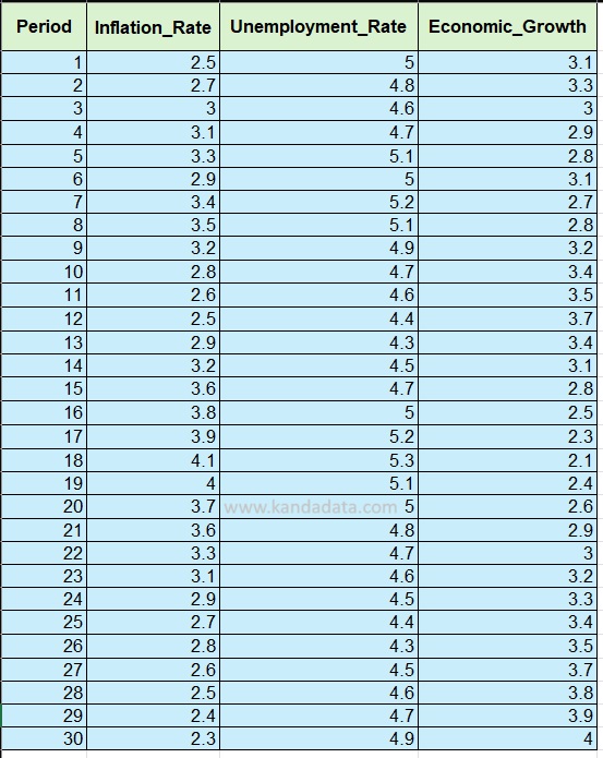
As practice for this tutorial, I’ll provide a case study. In this case study, a researcher wants to examine the effect of the inflation rate and unemployment rate on economic growth.

This example indicates that we will be using multiple linear regression analysis with two independent variables. A total of 30 data points have been collected for this exercise. The complete data can be seen in the table below:

Steps to Display Residual Values in Excel

Next, we will display the residual values from the data in the table above. The first step is to make sure that the Data Analysis Toolpak is enabled in your Excel. If it’s enabled, when you click the “Data” ribbon, you’ll see the “Data Analysis” option in the top right corner.

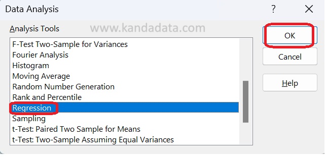
If that menu is not visible, you need to enable the Data Analysis Toolpak first. Once enabled, click on the “Data Analysis” menu. A list of available analysis tools will appear. Select “Regression,” as shown in the image below:

A new window will appear, prompting you to enter the data for the variables you’re using. In the “Input Y Range,” select the label and all the data for the economic growth variable. Next, for the “Input X Range,” select the labels and all data for the inflation rate and unemployment rate variables.

Then, check the “Labels” box and the “Confidence Level 90%” box. Under Output Options, choose where you want the results to be displayed. Now we come to the most important step — how to display the residual values.

To automatically display residual values in Excel, check the “Residuals” box. Once everything is set, click OK. You can see the detailed steps in the image below:

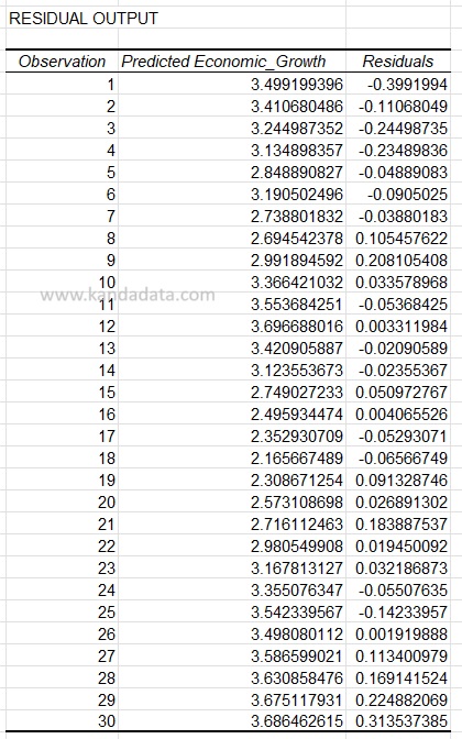
You will then see the results of the linear regression analysis in Excel. The output will be displayed in the location you specified earlier. Scroll down to the bottom of the results, where you’ll find a table containing the predicted Y values and the residuals. The residual values are shown in detail in the image below:

Now, you’ve successfully and easily obtained residual values in Excel! We hope this tutorial from Kanda Data is useful. See you in the next article!