Blog
Step-by-Step Tutorial: Finding Predicted and Residual Values in Linear Regression with Excel

In linear regression analysis, residual values play an important role in supporting the main analysis. Residual values are the difference between actual values and predicted values. In the assumption testing of linear regression using the OLS method, residual values are needed for the testing of assumptions.
One example is in the ordinary least squares (OLS) linear regression analysis, where one of the required assumptions is that the residuals are normally distributed. To test for normality, researchers must first find the residual values.
To find the residual values, researchers need the predicted values of Y from the linear regression equation. Researchers can calculate the predicted values of Y if they already know the estimated coefficients of the intercept and each independent variable.
If calculations are done manually, researchers would need to calculate the intercept and estimated coefficients of each independent variable first. Then, they can create an estimated equation using linear regression.
Based on the estimated equation of linear regression, researchers can then calculate the predicted values of Y by inputting each actual value of X one by one. After obtaining the predicted values of Y for all observations, researchers can then calculate the residual values of each observation. Residual values are obtained by subtracting the actual value of Y from the predicted value of Y.
Residual values can be calculated manually, but they can also be easily and quickly obtained using Excel. Given the importance of finding the predicted values of Y and residual values, in this tutorial, Kanda Data writes a guide on how to find the predicted values of Y and residual values in linear regression using Excel.
Example of a mini research case study
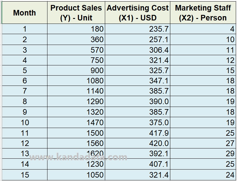
A researcher wants to know the influence of advertising costs and marketing staff on product sales. The researcher uses monthly time series data with a total of 15 observations.
Product sales are measured in units and are used as the dependent variable, while advertising cost measured in USD and marketing staff measured in persons are used as the independent variables. The data collected by the researcher can be seen in the table below:
Data Analysis Menu in Excel
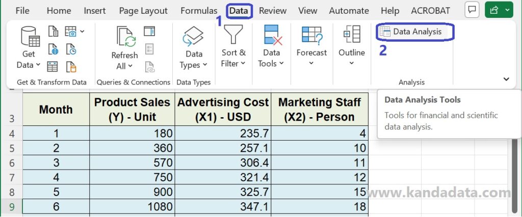
To find the predicted values of Y and residual values in Excel, the Data Analysis menu can be used. To access the Data Analysis menu, the researcher must first open the Excel file. After opening the Excel file, the researcher should click on the Data menu in Excel. In the upper right corner, the researcher will find the Data Analysis menu, as shown in the image below:
If the Data Analysis menu is not available in the upper right corner, the researcher needs to activate the Data Analysis Toolpak first. Please read the tutorial in the previous article titled: “How to Enable Data Analysis Button for t-test in Excel“.
Step-by-Step Tutorial on how to find Y predicted and residual values in Excel
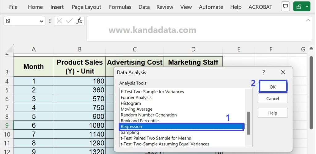
After clicking on the Data Analysis option located in the upper right corner of the Excel Data menu, the Data Analysis window will appear. To find the Y predicted and residual values, the researcher needs to select Regression from the available analysis tools in Excel, as shown in the figure below:
Next, after clicking OK, the Regression window will appear. At this stage, the researcher is asked to input all the data for both dependent and independent variables.
In the Input Y Range option, the researcher is required to input all the dependent variable data, including its label. Then, in the Input X Range option, the researcher needs to input all the independent variables along with their labels. The detailed steps are shown in the figure below:
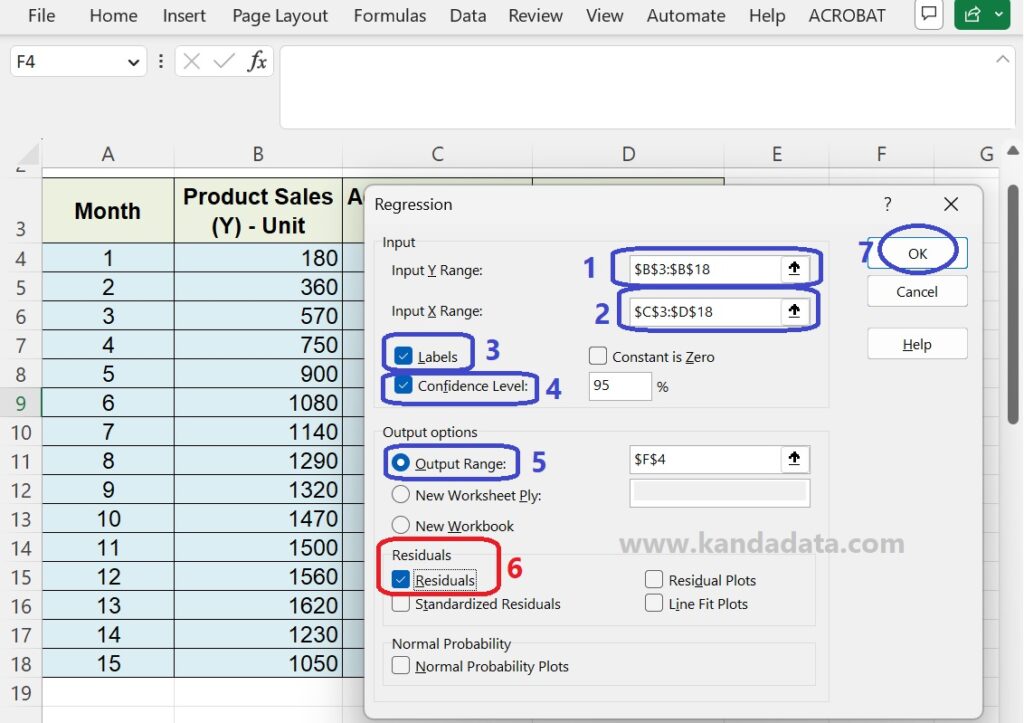
Next, don’t forget to enable Labels and enable the confidence level. In this study, the alpha value is set at 5%, so the researcher needs to write 95%. The alpha value can be adjusted according to the error limit set by the researcher in the study.
Finally, the output can be saved in the same Excel sheet, a different Excel sheet, or a new Excel file. In the example figure above, I have shown how to save the output in the same Excel sheet.
Based on the figure above, point number 6 (in red) is the crucial point that will determine whether the Y predicted and residual values will be displayed or not. To display the Y predicted and residual values, the researcher must enable the residual option.
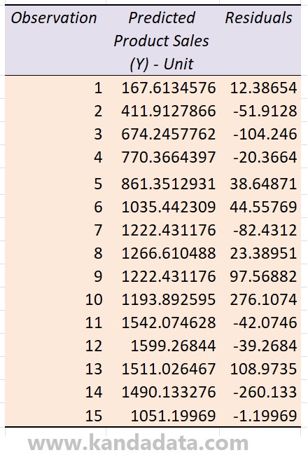
Y predicted and residual output
After following the step-by-step tutorial, the predicted value of the dependent variable and the residual value will appear on the same Excel sheet. The output shows the predicted values of the dependent variable and its corresponding residuals. The detailed output can be seen in the table below:
This is a step-by-step tutorial on how to find Y predicted and residual values in Excel. Hopefully, this tutorial can be useful and provide new insights for those who need it. See you in next week’s article. Thank you.