KANDA DATA

The Ordinary Least Squares (OLS) method in simple linear regression analysis is a statistical technique aimed at understanding the influence of an independent variable on a dependent variable. In simple linear regression, there is only one dependent variable and one independent variable.

In simple linear regression, the regression line can be represented mathematically as follows:

Y = bo + b1X + e

Where:

Y = dependent variable

X = independent variable

bo = intercept

b1 = regression estimate coefficient for variable X

e = disturbance error

The Ordinary Least Squares (OLS) method is a technique used to determine the optimal values of b0 and b1. In linear regression using the OLS method, this is done by minimizing the sum of the squares of the differences between the actual Y and the predicted Y.

Normality Assumption Test in Linear Regression Analysis

In simple linear regression analysis using the OLS method, a crucial next step is checking the normality of the residual distribution. Residuals are the differences between actual observation values and values predicted by the regression model.

The purpose of testing the normality of residuals is to ensure that they are normally distributed. This is important because many statistical methods require the assumption that data are normally distributed.

In linear regression equations, testing the normality of residuals is done to ensure that the parameter estimates and significance tests produced are reliable. This allows for accurate and scientifically accountable interpretation and conclusion.

Common normality tests used by researchers include the Kolmogorov-Smirnov test and the Shapiro-Wilk test. In this article, we will focus on the Shapiro-Wilk test, which is often used for relatively small samples.

Decision Criteria for Normality Testing in Regression

To aid researchers in decision-making based on normality test results, statistical hypotheses are set as follows:

Null hypothesis (Ho) = Residuals are normally distributed

Alternative hypothesis (H1) = Residuals are not normally distributed

Next, researchers need to determine the significance level alpha, typically set at 0.05. The decision criteria are then as follows:

If the p-value < 0.05, reject Ho (accept H1)

If the p-value > 0.05, accept Ho

How to Conduct a Normality Test using R Studio

Ensure you have installed and loaded the necessary packages for normality testing in R Studio. Packages commonly used include ‘car’ for normality testing functions (qqPlot), and ‘lmtest’ for calculating residuals from the regression model. The commands are as follows:

install.packages(“car”)

install.packages(“lmtest”)

library(car)

library(lmtest)

Next, perform the regression analysis first. Use the data we have discussed in the previous article, titled “Simple Linear Regression Analysis Using R Studio and How to Interpret It”. The data we use is detailed in the table below:

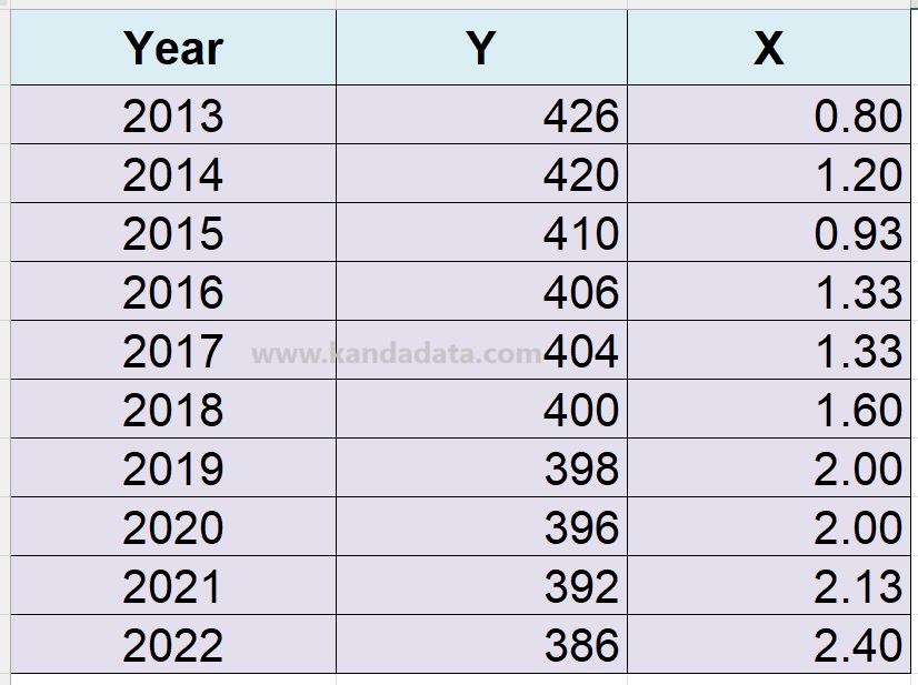
Use the lm() function to create a linear regression model. For example, model <- lm(y ~ x, data = dataset), where y is the dependent variable, x is the independent variable, and dataset is the data we use. The detailed command is as follows:

Model <- lm(Y ~ X, data = Regression)

After typing the above command, calculate the residuals using the resid() function, which can be detailed as follows:

Residuals <- resid(model)

Then, to test the normality of the residuals obtained using the Shapiro-Wilk test, simply type the following command:

shapiro.test(resid(model))

Output of Shapiro-Wilk Normality Test and How to Interpret the Results

Based on the normality analysis results performed as described above, the output is as follows:

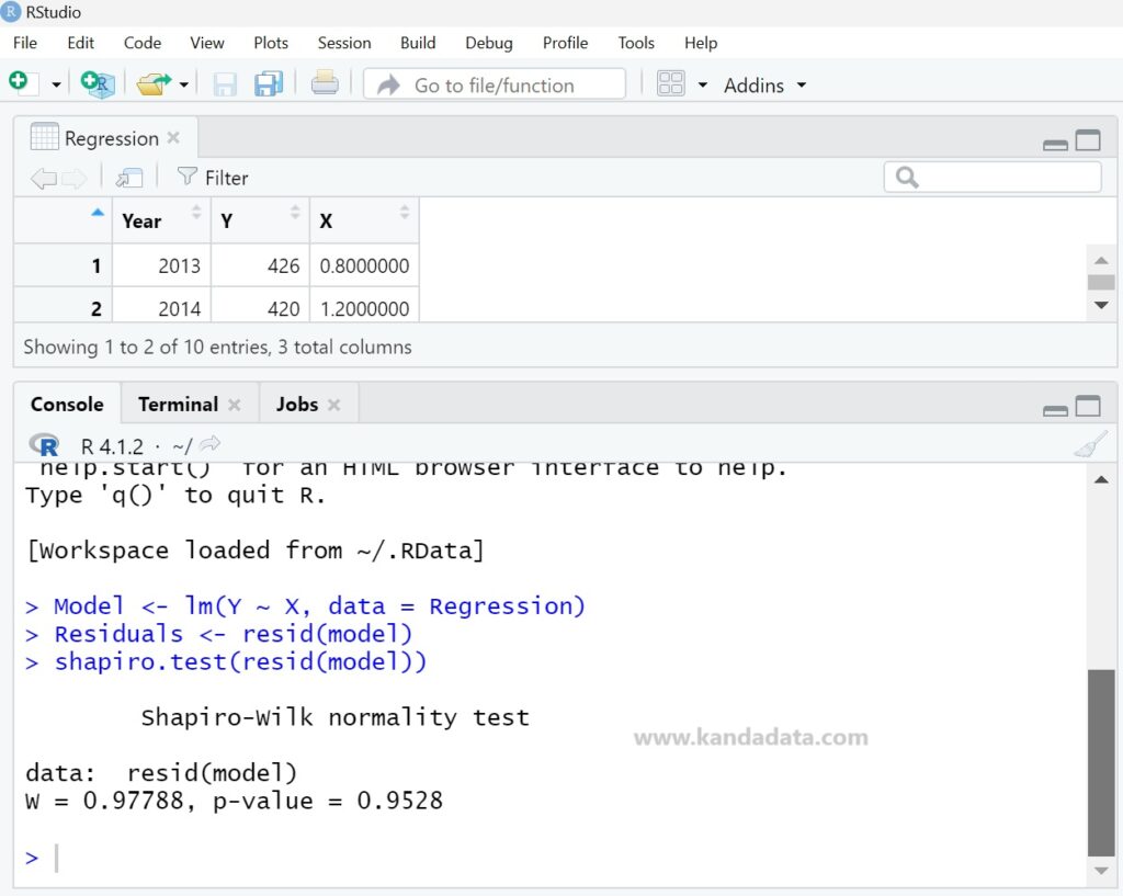
From the output, the test statistic (W) = 0.97788 and the p-value = 0.9528. Since the p-value is greater than 0.05, we accept the null hypothesis (H0). Therefore, we can conclude that the residuals are normally distributed.

That’s all for this article. I hope it is helpful and provides new insights for those who need it. Stay tuned for next week’s article update from Kanda Data.