KANDA DATA

The objective of the heteroscedasticity test is to determine whether the variance of residuals is constant. One of the assumption tests in linear regression using the ordinary least square (OLS) method is that the variance of residuals is constant.

The assumption of constant residual variance is called homoscedasticity. On the other hand, if the variance is not constant, it is called heteroscedasticity. Therefore, the assumption that must be fulfilled is homoscedasticity (non-heteroscedasticity).

The non-heteroscedasticity assumption must be fulfilled to obtain the best linear unbiased estimator. In the heteroscedasticity test, you also recommend formulating the hypothesis first. We can create a null hypothesis and an alternative hypothesis for the heteroscedasticity test.

The hypothesis for the heteroscedasticity test can be created as follows:

Ho: Residual variance is constant (homoscedasticity)

H1: Residual variance is not constant (heteroscedasticity)

Previously, do you still remember what residual is? Residual is the difference between the actual Y and the predicted Y variables. Residuals are used on the sample data. If you use population data, then we call it “error.”

On this occasion, I will test for heteroskedasticity using the Breusch Pagan test. In the test criteria, I will set an alpha of 0.05, then the criteria for testing the hypothesis are:

P-value > 0.05: Ho is accepted

P-value ≤ 0.05: Ho is rejected (H1 is accepted)

Heteroscedasticity Test Using Mini-Research Data

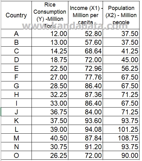
An example of a mini-research used on this occasion aims to determine the effect of income and population on rice consumption. In the mini-research, income and population were used as independent variables, and rice consumption was used as the dependent variable.

The data of our mini-research for exercise can be seen in the table below:

How to test for heteroscedasticity of Breucsh-Pagan in STATA

In the first step, you open the STATA and select the table icon with a pencil drawing (Data Editor). In the next step, you input all the data I have conveyed above.

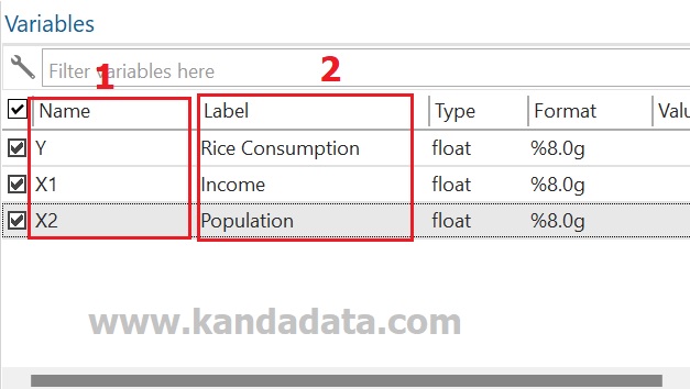
Data from the rice consumption variable (Y) is inputted in the first column, then data from the income (X1) and population (X2) variables are entered in the 2nd column and 3rd column. Next, you create the name and label the variable on the top right, as shown below:

To conduct the heteroscedasticity test, you type in the command in STATA as follows:

regress Y X1 X2

Next, you can press enter, and test the heteroscedasticity using Breusch-Pagan, then you type in the command in STATA as follows:

estat hettest

Next, you can press enter, and the heteroscedasticity test results using Breusch-Pagan will appear.

Heteroscedasticity Test Output and How to Interpreting the Output

The output of the heteroscedasticity test based on the results of the analysis using STATA can be seen in the table below:

Based on the heteroscedasticity test output according to the table above, the prob>chi2 value is 0.3482. Based on the hypothesis that has been created previously, the results of hypothesis testing indicate that the null hypothesis is accepted (p-value is greater than 0.05). Thus it can be concluded that the residual variance is constant (homoscedasticity).

Because the residual variance is constant (homoscedasticity), the regression model has fulfilled the OLS assumption. To better understand heteroscedasticity and how to address it in linear regression, I highly recommend the book Econometric Analysis. Well, that’s the article on this occasion that kanda data can convey for all of you. I hope this article will be beneficial for us. See you in the next article!