Researchers often choose linear regression analysis to determine the effect of the independent variable on the dependent variable. Simple linear regression was used to analyze the regression model with only one independent variable. There are many benefits of using simple linear regression analysis. Based on that, Kanda Data on this occasion will share a simple linear regression analysis tutorial and how to interpret the output in SPSS.
In simple linear regression analysis, several assumptions must be met. If a regression model has passed the assumption test, such as the normality test, heteroscedasticity, linearity, and others, the model estimation will be consistent and unbiased. We can call it the Best Linear Unbiased Estimator (BLUE). Some reference sources, this assumption test is often also called the Gauss Markov assumption.
On this occasion, I will give an example of a case study that will be analyzed using simple linear regression. It is easier for you to understand the application of linear regression analysis and how to interpret the results.
For example, in a case study, a company “ABC” manager in a city “XYZ” was asked by the company’s owner to increase the selling price of bread in his company. Surely there will be an impact from the price increase, the manager thought. Therefore, the manager will analyze to find out how the influence of the selling price of bread on the number of bread sales.
The manager then collected ten years of price and sales data. We can call the collected data time-series data. A simple linear regression analysis was carried out to answer the manager’s question. The measured variables consist of the selling price of bread as the independent variable (X) and the number of bread sales as the dependent variable (Y). In this case, we will use simple linear regression analysis, where there is only one independent variable.
The data that has been collected will be processed using SPSS. SPSS consists of two windows, namely “Data View” and “Variable View”. Data collected previously can be directly input in the data view window. How to input data into SPSS can be input directly into the application or copy-paste data from Microsoft Excel.
Next, open the “Variable View” window. Fill in the name with “Y” and fill in the label column with “Bread Sales”. Next on the second line, fill in the name with “X” and fill in the label column with “Selling Price”. Neither variable has decimal values so that the decimal column can be omitted. Next, fill the measure column with a scale to indicate that the data measurement scale is interval/ratio. We have successfully input the data and are ready to start the simple linear regression test.
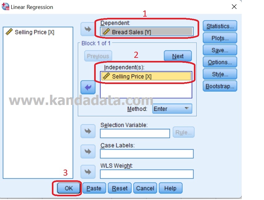
From the various menu options available in SPSS, please click the “analyze” menu, then click “regression” and then click “linear”. Then a new window will appear “Linear Regression”. Move the bread sales variable (Y) into the dependent box and the selling price (X) variable into the independent box. Ignore the other options, then click Ok. This step can be seen in more detail in the image below:
Not long ago, a simple linear regression analysis output appeared. Now is the time for us to interpret the regression analysis output that we have tested. In interpreting the regression output, the first thing to look at is the R Square value in the model summary, as shown in the following figure:
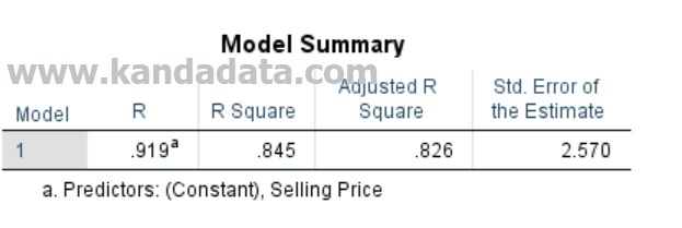
Based on the model summary output, we see the value of R Square. This value indicates whether the model is good or not. We can see the value of R square is 0.845. We can interpret this value that the variation of the bread sales variable of 84.5% can be explained by the variation of the selling price variable. The remaining 15.5% is explained by variations of other variables not explained in this model.
Next, we interpret the output for the F test and t-test as shown in the image below:
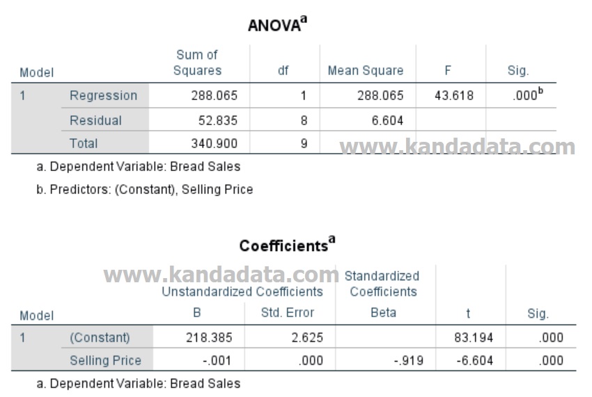
Based on the picture, we interpret the F test value. The F test value is 43,618 with a P-Value value less than 0.05, meaning that simultaneously the selling price variable has a significant effect on bread sales. Furthermore, we interpret the value of the t-test. The coefficient value of the selling price variable is -0.001 with a p-value less than 0.05, meaning that partially selling price has a significant effect on bread sales. The selling price coefficient is negative, meaning that every increase in selling price will decrease bread sales.
For those of you who are more interested in learning to use audio-visuals, you can watch the following video:
Before we end this article, we can conclude that the sale of bread has a statistically significant effect on the number of bread sales. Based on the negative regression coefficient, it indicates that if the manager increases the selling price, it will decrease bread sales. The higher the price is raised, the potential to reduce the number of sales is getting bigger. The manager needs to do further research to determine the best price increase that is still profitable for the company.
For a step-by-step guide to performing and interpreting simple linear regression in SPSS, I highly recommend the book How to Use SPSS®: A Step-By-Step Guide to Analysis and Interpretation. This user-friendly resource is ideal for both beginners and advanced users looking to master SPSS.
Alright, I guess we’ll end this article. Hopefully, this article is useful. See you in the next article update!