
In many parametric statistical tests, it’s assumed that the data must follow a normal distribution. That’s why, when we’ve gathered research data and are planning to use parametric statistical analysis, checking for normality is crucial. We need to make sure that the data follows a normal distribution before proceeding with further analysis.
However, sometimes the results show that the data doesn’t follow a normal distribution. One possible cause? Outliers.
In this article, Kanda Data explores how a single outlier can make your dataset appear non-normal, even if the rest of the data is perfectly fine.
The Link Between Outliers and Normality Tests
Before diving deeper, let’s first understand the basic concept behind the test. You may wonder, why choose one-way ANOVA?
As mentioned earlier, one-way ANOVA is the appropriate test when you’re comparing the means of more than two sample groups. Normally, if you’re comparing two groups, you’d use a paired t-test or an independent t-test. But for more than two groups, one-way ANOVA is the recommended approach to determine whether significant differences exist among the group means.
Assumptions of One-Way ANOVA
As mentioned earlier, testing for normality is a key step to ensure that the assumptions for parametric tests are met. These assumptions help ensure that the estimates from the statistical tests are reliable and unbiased.
From our experience, outliers can significantly affect the results of a normality test. Even when most of the data looks fine, a few extreme values can skew the outcome.
For instance, when we test a dataset without outliers, it may pass the normality test. But once a few extreme values are included, the same dataset might suddenly fail the test.
Let’s walk through a simple case study to see how this works.
Case Study: Normality Test with and without Outliers
Imagine a researcher collects weight data from 15 participants. The data (in kilograms) is as follows:
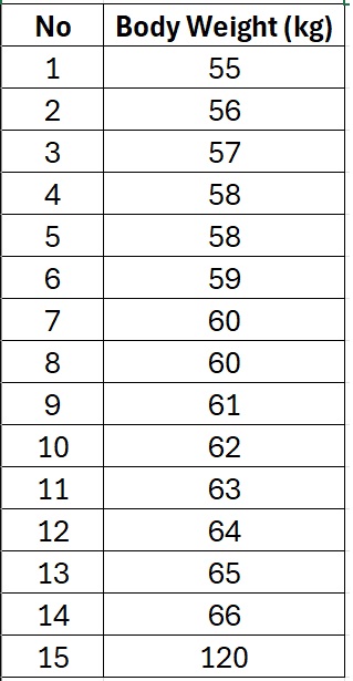
Most of the weights are between 55 and 66 kg, but one value stands out, 120 kg. This is clearly an outlier. The output of Shapiro-Wilk normality test using SPSS is as follows:
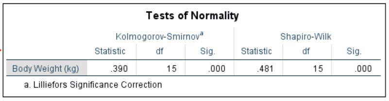
Running a Shapiro-Wilk normality test (in this case using SPSS) reveals a p-value < 0.05, which means the data is not normally distributed.
If we plot the data, we’ll notice that the distribution is skewed to the right, and that skewness is mainly due to the presence of the 120 kg outlier.
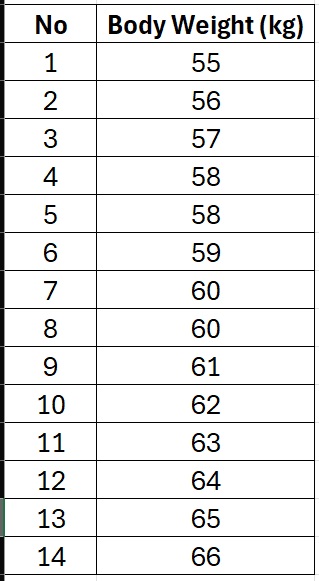
What Happens If the Outlier Is Removed?
Now, let’s see what happens if we remove the 120 kg outlier. Updated dataset is as follows:
Running the same normality tests again using Shapiro-Wilk normality test, we now find:
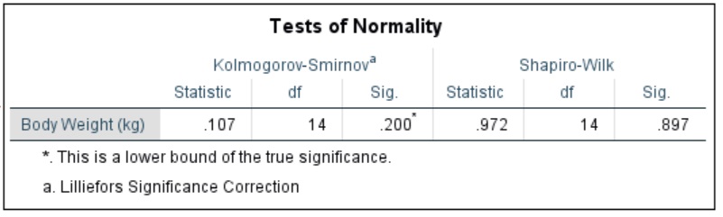
Based on the test, we obtain p-value > 0.05, so we can concluded that the data is normally distributed.
How to Detect Outliers
In our example, detecting the outlier was simple since the sample only had 15 data points. But what if you’re analyzing hundreds or thousands of records? Here are some practical methods to detect outliers:
Firstly, You can use visual tools such as Boxplots, scatterplots, or histograms to help you spot extreme values easily. Secondly, apply statistical methods using calculate Z-scores or use the interquartile range method to find values outside the lower and upper bounds.
Here’s how to deal with outliers in normality testing: (a) Identify and evaluate outliers: Are they valid observations or errors?; (b) Run two analyses: Compare results with and without the outliers; (c) Consider using non-parametric tests, such as Mann-Whitney U or Kruskal-Wallis, if you decide to keep the outliers in your dataset. Remember, outliers are few, but their impact can be massive, especially in normality testing.
So, can one outlier ruin your normality test? Absolutely. That’s why it’s important to always check for outliers before making any statistical decisions.
I hope this article from Kanda Data helps you gain new insights into data analysis. Stay tuned for more tips and tutorials!
