
When analyzing statistical data, such as evaluating the variability of rice yields among different farmers, standard deviation is a primary indicator of how far the data spreads from the mean. While Excel provides instant functions like =STDEV.S(), calculating it manually (step-by-step) builds a much stronger understanding of your data’s underlying structure.
This foundational knowledge is especially valuable when writing robust, transparent methodology sections for high-impact international journals. In this article, Kanda Data will guide you to calculate manually using Excel. Let’s explore how to perform this transformation and calculation using a step-by-step method in Excel, using a sample dataset of rice production from 25 farmers.
The Sample Standard Deviation Formula
Mathematically, the formula for sample standard deviation (s) is:
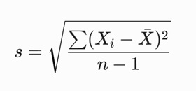
Where: Xi = The i-th data value (Rice Production); Xbar = The sample mean; n = Total number of sample observations.
Step-by-Step Excel Calculation
Step 1: Prepare the Data Structure
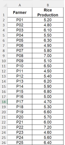
Enter your raw data into Excel columns. Use the following structure:
- Column A: Farmer ID (P01 to P25)
- Column B: Rice Production (Ton/Ha). This is our X variable.
Step 2: Calculate the Mean
Before finding the deviations, you must determine the average of the entire sample.
- Below the last row of data (e.g., cell B27), enter the formula: =AVERAGE(B2:B26)
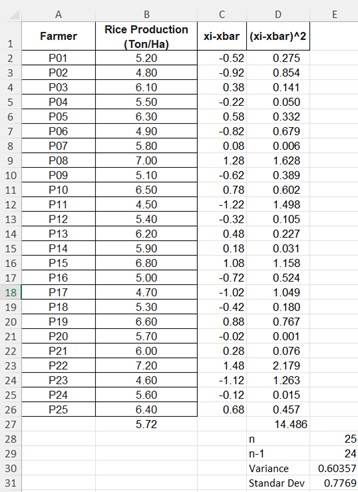
- This formula sums all rice production values and divides by 25. The mean for this dataset is 5.72 Ton/Ha.
Step 3: Calculate Individual Deviations
This step measures how far each farmer’s yield deviates from the regional average.
- Create a new column header in cell C1: Deviation (xi-xbar).
- In cell C2, enter the formula: =B2-$B$27 (Ensure you use the $ signs to lock the mean cell reference so it does not shift when copied).
- Drag or double-click the fill handle at the bottom right corner of cell C2 to copy the formula down to cell C26.
Step 4: Square the Deviations
Because some deviation values will be negative, we must square them to ensure all values are positive.
- Create a new column header in cell D1: Squared Deviation ((xi-xbar)^2).
- In cell D2, enter the formula: =C2^2.
- Copy this formula down to row D26.
Step 5: Calculate the Sum of Squared Deviations
Next, sum all the values in the Squared Deviation column.
- In cell D27 (aligned with the totals row), enter the formula: =SUM(D2:D26).
- The result of this addition is known as the Sum of Squares (SS).
Step 6: Calculate the Sample Variance
Variance is the average of the squared deviations. Because we are working with sample data, the denominator is the degrees of freedom, which is n – 1 (25 – 1 = 24).
- In cell D30, write the label Sample Variance.
- In cell E30, enter the formula: =D27/24.
Step 7: Calculate the Sample Standard Deviation (Square Root of Variance)
The final step is to extract the square root of the variance to return the data to its original unit (Ton/Ha).
- In cell D31, write the label Manual Standard Deviation.
- In cell E31, enter the square root formula: =SQRT(E30)
Verification with Excel’s Automated Formula
To ensure your manual calculation is perfectly accurate, use Excel’s built-in formula in an adjacent cell to double-check:
=STDEV.S(B2:B26)
The result from the manual step-by-step calculation above will yield the exact same value as the automated formula, which is approximately 0.7769 Ton/Ha.
Ok, thank you for read this article. See you in the next article from Kanda Data.
