Blog
Handling Non-Normally Distributed Data by Removing Outliers
The topic I’m writing about today is prompted by questions on how to handle data that is not normally distributed. We know that in quantitative analysis, several statistical tests require that the data be normally distributed. This is an interesting topic that we will delve deeper into in this article.
In quantitative data analysis, one of the commonly used assumptions is that the data is normally distributed. A normal distribution, when understood more deeply, can be observed in data forming a symmetrical bell curve. On this bell curve, most values will be centered around the mean.
However, in reality, the results of normality tests do not always match our expectations. In some cases, we may encounter issues where the data is not normally distributed.
Based on experience in conducting a series of analyses and data processing, one of the causes is the presence of outliers in our data. The presence of outliers or data points that significantly differ from the majority of the data can impact the results of normality tests.
These outliers can cause biased data interpretation, even in descriptive statistical analysis. Therefore, identifying and addressing outliers is an essential step in data analysis.
This article will discuss how to handle non-normal data by removing outliers. I will provide a case study example to help readers better understand the concept.
Assumption of Normally Distributed Data
As mentioned earlier, several quantitative analyses require normally distributed data. For example, researchers using t-tests, ANOVA, and linear regression require normally distributed data to ensure consistent and unbiased estimation results.
In normally distributed data, the data spread forms a symmetrical bell curve around the mean. Most normally distributed data lie within a standard deviation close to the mean.
If the data is not normally distributed, the analysis results can become invalid and biased. Therefore, it is important for us to evaluate whether the data meets the normal distribution assumption according to the statistical test we choose.
Solutions for Non-Normally Distributed Data
At the beginning, I mentioned that outliers are data points that significantly differ from most data. Thus, removing outliers is an effective method to make data closer to a normal distribution.
The first step is to identify and detect outliers. The easiest way to identify outliers is through descriptive statistical tests, including mean, median, and standard deviation. We can mark data points with large standard deviations or those significantly different from the mean as potential outliers.
We can also visualize data using boxplots and observe data points outside the whiskers. Additionally, we can calculate the Z-score to identify outliers in our dataset.
Outliers can be removed or replaced with new data following scientific principles. Outliers may arise due to incorrect sampling techniques or errors during questionnaire completion. Therefore, validation and verification by researchers are crucial steps.
In cross-sectional data, we can remove outliers or replace them with new respondent data. If outliers are due to errors or are irrelevant to the analysis, they can be removed from the dataset. However, it is important to justify or provide reasons for the removal of these outliers.
Case Study and Interpretation
To provide a clearer picture, we will conduct a case study with cross-sectional data consisting of 30 observations. Suppose we have a dataset containing weekly sales values from 30 stores. The data can be seen in the table below:
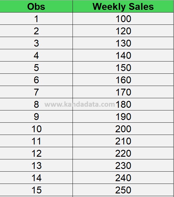
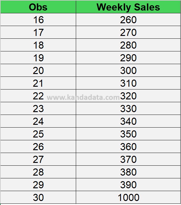
Based on the above data, we know that in the last observation, there is a value significantly higher than most weekly sales data from other stores. This data point is likely an outlier.
Normality tests will be conducted using the Kolmogorov-Smirnov and Shapiro-Wilk tests with the results shown in the image below:
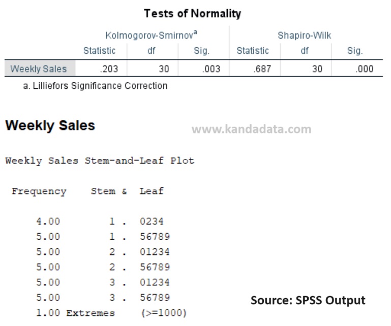
Based on the analysis results, it is known that according to both tests, Kolmogorov-Smirnov and Shapiro-Wilk, the p-value < 0.05. This indicates that the null hypothesis is rejected (accepting the alternative hypothesis) which means the data is not normally distributed.
In the output below, we also know that the value of 1000 is an extreme outlier. Therefore, this outlier is suspected to cause the data to be not normally distributed.
Now let’s try removing this outlier. We will see how removing the outlier impacts data normality.
After removing the outlier, it is expected that the mean and median values will be closer and show a more normal data distribution. The results of the normality test using Kolmogorov-Smirnov and Shapiro-Wilk tests using SPSS are shown in the image below:
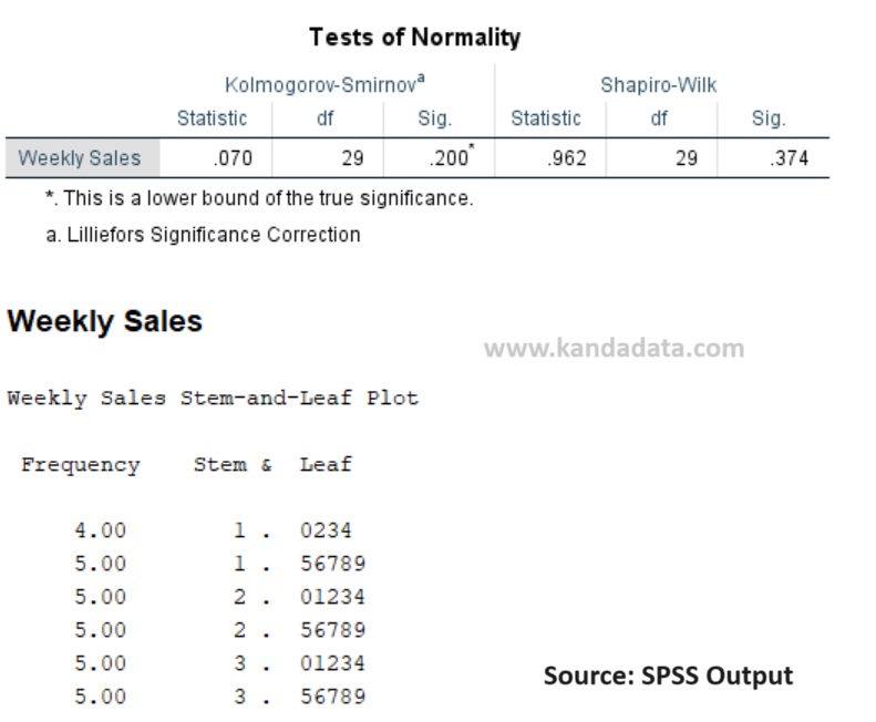
Based on the output above, after removing the outlier, the Kolmogorov-Smirnov test p-value is 0.200 and the Shapiro-Wilk test p-value is 0.374. Based on these results, both p-values are > 0.05, indicating that the null hypothesis is accepted, meaning the data is normally distributed.
Additionally, the outlier test shows no extreme values. By removing the outlier, we achieve a data distribution closer to normal. This enables more valid statistical analysis and more reliable results. It is important to note that removing outliers should be done carefully and based on proper evaluation.
Conclusion
Handling non-normally distributed data is a crucial step in statistical analysis. Outliers often cause non-normal data distribution. By identifying and removing outliers, we can make the data closer to a normal distribution.
That concludes the article I can write for this occasion. I hope it is useful and adds knowledge value for readers in need. See you in the next educational article from Kanda Data!