Blog
How to Calculate Durbin Watson Tests in Excel and Interpret the Results

Researchers who use time series data in linear regression analysis with the OLS method need to conduct some of the required assumption tests. One of the assumption tests required in the regression is the autocorrelation test.
Autocorrelation tests can be done in both simple and multiple linear regression. The autocorrelation test aims to test whether there is a correlation between residuals in the t period and the previous period (t-1) in the linear regression model. If there is a correlation, then it is called an autocorrelation problem.
The autocorrelation test must be conducted to obtain the best linear unbiased estimator. One thing that needs to be considered by researchers is that the autocorrelation test is conducted on time series data. In comparison, cross-section data does not need to be tested for autocorrelation.
Several ways can detect autocorrelation, including Durbin Watson test, Lagrange multiplier test, Breusch Godfrey test, and rank test. On this occasion, Kanda Data will discuss the Durbin-Watson autocorrelation test.
Durbin Watson Test on mini research
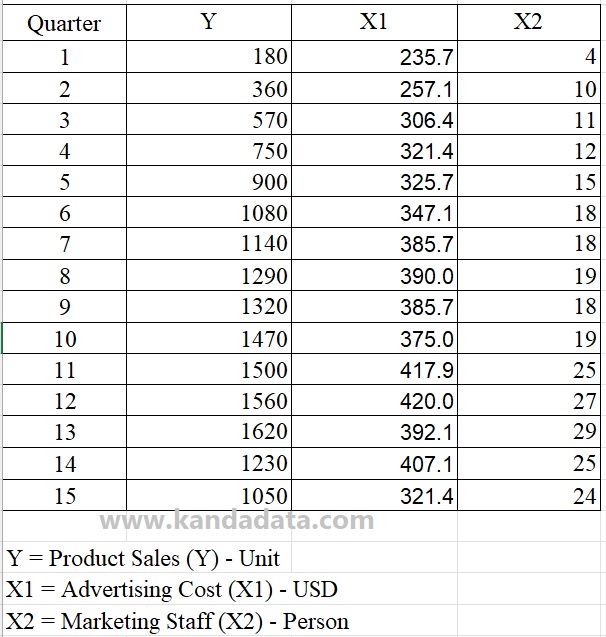
I have prepared mini research materials as a practice for the Durbin Watson test. Based on the case examples, the researcher aims to determine the effect of advertising costs and marketing staff on product sales. Researchers took quarterly time series data from as many as 15 observations.
Based on the data that has been collected, the researcher then specifies the equation as follows.
Y = b0 + b1X1 + b2X2 + e
Y = Product sales – Units (dependent variable)
X1 = Advertising Cost – USD (independent variable)
X2 = Marketing Staff – Person (independent variable)
b0 = Intercepts
b1, b2 = Regression estimation coefficients
e = residuals/errors
Based on the specifications of the equations that the researcher has prepared, the researcher inputs the data collected in Excel. In detail, the data that researchers have collected can be seen in the table below:
The Formula for Calculating Durbin Watson Statistics
The formula used to calculate the statistical Durbin-Watson value includes several components that need to be calculated first, namely predicted Y, residual (et), the difference between the residuals in period t and the previous period (et – et-1), residual squared (et^2), and (et – et-1)^2. Durbin Watson statistics were obtained by dividing the squared residual value (et^2) by (et – et-1)^2.
It will be easier to make a calculation template using Excel to calculate the Durbin-Watson statistics. In detail, the template for calculating the Durbin-Watson statistics can be seen in the table below:

How to find Predicted Y and Residual values in Excel
Researchers can easily calculate the predicted Y and residual values in excel. Predicted Y can only be calculated if the estimated coefficients bo, b1, and b2 have been obtained.
To manually calculate the estimated coefficients bo, b1, and b2, you can read my previous article entitled: “Finding Coefficients bo, b1, b2, and R Squared Manually in Multiple Linear Regression“.
Furthermore, you only need to subtract the actual Y value with the predicted Y to calculate the residual value. However, there is an easy and fast way that researchers can use to find the predicted Y and residual values in excel.
You can use the analysis data toolpak in Excel. You can click “Data”, then in the upper right corner is an option “Data Analysis”. If you cannot find it, please activate the data analysis toolpak following my tutorial article entitled: “How to Activate and Load the Data Analysis Toolpak in Excel“.
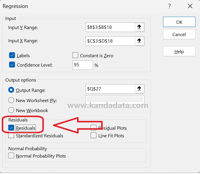
In the next stage, you click regression from several analysis tools provided by Excel. After clicking regression, a new window will appear. Then input all variable Y data, including its label, to “Input Y Range”. In the same way, input all data of variable X, including its label, to “Input X Range”.
Enable labels and set confidence levels to 95%. You can save analysis results in the same sheet, new worksheet ply, or new workbook. One important thing that needs to be done is to enable “Residuals”.
If you have activated “Residuals”, the predicted Y and residuals will appear in the analysis results. In detail, the steps to bring up the predicted Y and residuals can be seen in the image below:
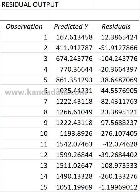
After you click OK, then the analysis output will appear. Based on this output, you will find the predicted Y and residuals at the bottom, as shown below:
How to Calculate Durbin Watson Statistics in Excel
Based on the Durbin Watson test calculation template using excel, the predicted Y and residual values can be directly inputted into the calculation template.
To calculate the value of et – et-1, you only need to reduce the residual value in period t (et) with the residual in the previous period (et-1). In detail, how to calculate using excel can be seen in the image below:

Based on the picture above, to calculate et^2, you only need to square the residual value. The same thing is also done to calculate the value of (et – et-1)^2 by squaring the value of et – et-1.
Next, you can copy and paste all calculation results for all observations. In detail, the results of the calculation of the components of the Durbin-Watson statistical formula can be seen in the image below:
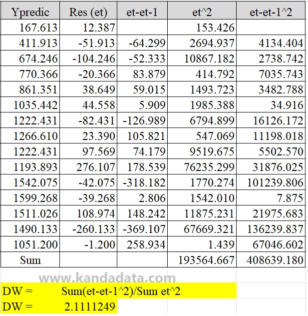
Based on the picture above, the Durbin Watson statistical calculation formula:
Durbin Watson Statistics (DW) = Sum(et-et-1^2)/Sum et^2
Durbin Watson Statistics (DW) = 408639.180/193564.667
Durbin Watson Statistics (DW) = 2.1111249
Durbin Watson interpretation
After knowing the value of Durbin-Watson statistics, the next step is the interpretation of Durbin Watson. To conclude whether there is autocorrelation, researchers can compare the Durbin-Watson statistics with the Durbin-Watson table.
Here I will give an example of the Durbin-Watson table with an alpha of 5%. Durbin Watson table with alpha 5% can be seen in the image below:

Based on the picture above, to read the Durbin-Watson table, researchers need to know that the column shows the number of independent variables and the row shows the number of observations.
Based on the mini-research example, it is known that the number of independent variables consists of 2, and the number of observations is 15. Therefore, k = 2 and n = 15. Thus, dL = 0.9455 and dU = 1.5432 are obtained.
The next step, to make it easier to draw conclusions from the autocorrelation analysis using the Durbin-Watson test, the researcher can make a graph like an image below:

The researcher must calculate the 4-dU and 4-dL values according to the picture above. The Durbin-Watson statistical value of 2.11112486 is between 1.5432 (dU) and 2.4568 (4-dU). Based on the graph, it can be concluded that the regression equation has no autocorrelation.
To learn more about statistical tests like the Durbin-Watson test and other essential methods, I recommend the book Practical Statistics for Data Scientists: 50+ Essential Concepts Using R and Python. This book provides practical insights into statistical techniques with real-world applications in data science.
It is an article that I can write for all of you on this occasion. Hopefully useful for all of you. Wait for the article update next week. Thank you!