KANDA DATA

One of the assumptions required in Ordinary Least Squares (OLS) linear regression is that the variance of the residuals is constant. This assumption is often referred to as the homoscedasticity assumption. Some researchers are more familiar with the term heteroscedasticity test.

The expected result of the heteroscedasticity test is that there is no heteroscedasticity problem. Heteroscedasticity occurs if the variance of the residuals is not constant or if the variance of the residuals differs.

Furthermore, constant residual variance (homoscedasticity) is an expected assumption that needs to be fulfilled by researchers who analyze data, both cross-sectional and time-series data using OLS method. Therefore, it is necessary to perform a non-heteroscedasticity assumption test.

There are several methods that can be used to determine whether the residual variance is constant or not, and one of them is the Breusch-Pagan test using R Studio. This is part 3 of the tutorial discussing how to test heteroscedasticity and its interpretation in R.

Formulating the Heteroscedasticity Test Hypotheses

To test whether the residual variance is constant or not, researchers can formulate their statistical hypotheses. Statistical hypotheses can be formulated into null hypotheses and alternative hypotheses.

The statistical hypotheses and their acceptance criteria for the heteroscedasticity test in R can be formulated as follows:

Ho: p-value >0.05 = Homoscedasticity (constant residual variance)

Ha: p-value <0.05 = Heteroscedasticity (non-constant residual variance)

Sample Data for Heteroscedasticity Test

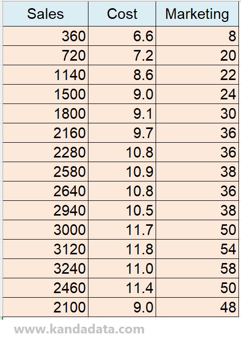
As practice material to understand how to test heteroscedasticity, I have prepared sample data for multiple linear regression. The purpose of the research is to determine the effect of costs and marketing on sales.

Therefore, costs and marketing are used as independent variables, and sales are used as the dependent variable. The data collected by the researcher can be seen in detail in the table below:

Importing Data from Excel to R Application

Importing data in R is done by clicking on the file, then from the various options available, click on import dataset. Since I have saved the data using Excel, choose from Excel.

The next step is for the researcher to browse the location where the Excel file is saved. Next, a preview of the data inputted in Excel will appear, then click import. If these steps have been done correctly and systematically, a preview of the imported data from Excel will appear in R Studio.

For researchers who want to learn how to test multiple linear regression and multicollinearity in OLS linear regression method, they can read the previous articles titled:

1. “Multiple linear regression analysis and interpretation in R (Part 1)”

2. “How to Analyze Multicollinearity in Linear Regression and its Interpretation in R (Part 2)“

The syntax for Testing Heteroscedasticity in R

To test for heteroscedasticity in R, researchers need to perform multiple linear regression analyses in R first. The first step that can be taken by researchers is to type the syntax for multiple linear regression analysis.

Syntax “Sales ~ Cost + Marketing” should be adjusted based on the number of variables used. Please pay attention to the capital and small letters of the variable label, type them exactly as they appear in the preview in R Studio.

Next, in the syntax “data = Multiple_Linear_Regression”, the data source used is specified. Please write it exactly as the file name used when importing data.

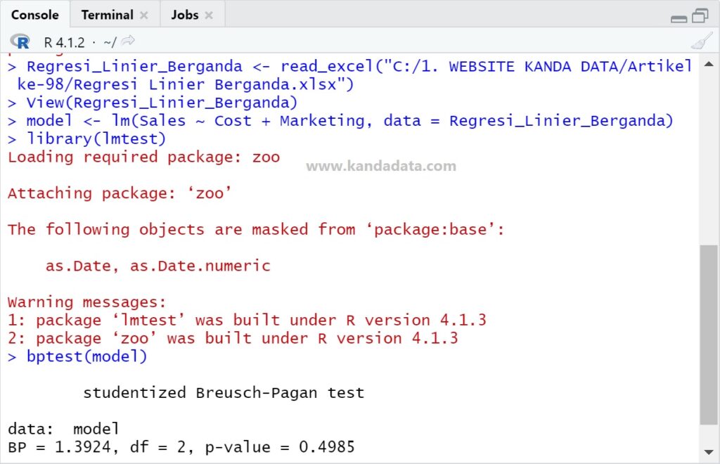
After pressing enter, the next step is to type “library(lmtest)”. Then type the syntax “bptest(model)”. This syntax is intended to display the results of the Breusch-Pagan test.

In detail, the syntax for testing heteroscedasticity and the output of the Breusch-Pagan test can be seen in the figure below:

Interpretation of Heteroscedasticity Test Output in R

The output of the Breusch-Pagan heteroscedasticity test in R is the same as other analysis tools. Based on the figure above, it can be seen that the Breusch-Pagan value was 1.3924.

Based on the output, the p-value was 0.4985. Then the acceptance criteria for the hypothesis are as follows:

Ho: p-value >0.05 = Homoscedasticity (constant residual variance)

Ha: p-value <0.05 = Heteroscedasticity (non-constant residual variance)

Based on the acceptance criteria, the p-value is greater than 0.05, so the null hypothesis is accepted. Since the null hypothesis is accepted, it can be concluded that the residual variance is constant (homoscedasticity).

Therefore, the regression equation fulfilled one of the assumptions of the OLS linear regression method, which is constant residual variance. This concludes part 3 of this article, and the next part will be available soon.