If you have ever tried to include categorical data—like gender, location, or ownership status—into a regression model, you might have hit a roadblock. Traditional regression models require numerical inputs, leaving many researchers wondering how to analyze qualitative factors.
The solution? Dummy variables.
In this tutorial, we will break down exactly what dummy variables are, how to set them up, and how to interpret the results using a practical dataset on rice production. Whether you are using STATA, SPSS, or Excel, mastering this concept will elevate the quality of your data analysis and research publications
What is a Dummy Variable?
A dummy variable (often called an indicator variable) is a numeric variable that represents categorical data. It takes the value of 0 or 1 to indicate the absence or presence of some categorical effect that may be expected to shift the outcome.
For example, if we want to measure the impact of land ownership on crop yield, we cannot type “Owned” or “Rented” into our statistical software. Instead, we assign a value:
1 = Owned Land
0 = Rented Land (This becomes our “reference” or “baseline” category).
The Dataset: Agricultural Economics Example
To make this concrete, let’s look at a sample dataset of 30 farmers. We want to understand what drives rice production. We have continuous variables (land area and fertilizer) and one categorical variable (land status).
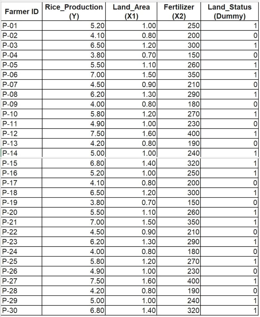
Here is the breakdown of our variables:
Dependent Variable (Y): Rice Production in Tons
Independent Variable 1 (X1): Land Area in Hectares
Independent Variable 2 (X2): Fertilizer applied in Kg
Dummy Variable (D): 1 for Owned Land, 0 for Rented Land
Formulating the Regression Model
When we introduce our variables into a multiple linear regression model, the equation looks like this:
Y = bo +b1X1 + b2X2 + b3D + e
Where: bo is the intercept, b1 and b2 measure the impact of land area and fertilizer on rice production, b3 is the coefficient for our dummy variable, and ϵ represents the error term.
How to Interpret the Dummy Variable Coefficient (b3)
Interpreting continuous variables like fertilizer is straightforward: “For every additional 1 Kg of fertilizer, rice production increases by X tons, holding other variables constant.”
But how do we interpret b3 (dummy variable)?
Because our dummy variable only moves from 0 to 1, b3 represents the average difference in rice production between farmers who own their land (1) and farmers who rent their land (0), assuming land area and fertilizer use are exactly the same.
If b3 is positive and statistically significant: It means farmers who own their land produce significantly more rice than those who rent. If b3 is negative and statistically significant: It means land ownership is associated with lower production compared to renting.
Why This Matters for Your Research
Including dummy variables allows researchers to capture the nuance of real-world scenarios. In agricultural economics, factors like access to credit, participation in farmer groups, or the adoption of new technology can all be quantified using this simple 0 and 1 framework.
Step-by-Step Tutorial: How to Run the Analysis in Excel
We will walk through how to run this regression analysis using popular statistical tools among researchers: Microsoft Excel.
- Prepare the Data: Enter the dataset exactly as shown in the table into a blank Excel worksheet.
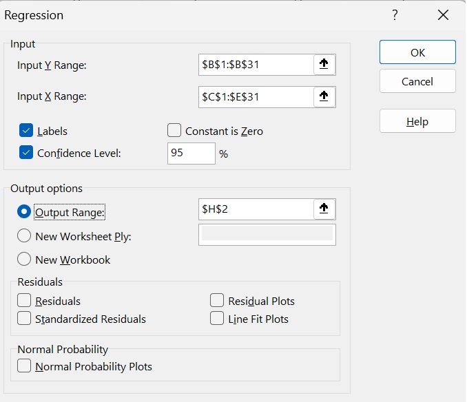
- Open the Tool: Go to the Data tab on your ribbon and click on Data Analysis. (Note: If you don’t see it, you may need to enable the Analysis ToolPak add-in in your Excel options).
- Select Regression: Scroll down, select Regression, and click OK.
- Input the Variables: * For the Input Y Range, select the entire column for Rice_Production (Y).
- For the Input X Range, select the columns for Land_Area (X1), Fertilizer (X2), and Land_Status (Dummy) simultaneously.
- Run the Model: Check the Labels box (if you highlighted the column headers), choose where you want the output to appear, and click OK.
Exact Results & Interpretation
Based on our specific dataset of 30 farmers, running this multiple linear regression yields the following actual output:
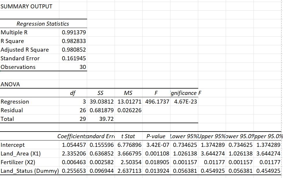
The Estimated Regression Equation: Y = 1.0545 + 2.3352(X1) + 0.0065(X2) + 0.2557(D)
What do these numbers actually mean in practice?
1. Model Accuracy (Goodness of Fit)
The Adjusted R-squared is 0.981. This is an exceptionally strong model, meaning that 98.1% of the variation in rice production is successfully explained by the combination of land area, fertilizer application, and land ownership status.
2. Interpreting the Continuous Variables
- Land Area (X1): The coefficient is 2.3352. This means that for every additional 1 hectare of land, rice production increases by an average of 2.3352 tons, holding all other variables constant. (Statistically significant at p < 0.01).
- Fertilizer (X2): The coefficient is 0.0065. This indicates that for every additional 1 kg of fertilizer applied, rice production increases by 0.0065 tons (or 6.5 kg), assuming land area and ownership status remain unchanged. (Statistically significant at p < 0.05).
3. Interpreting the Dummy Variable (D)
This is the core of our tutorial. The coefficient for our categorical dummy variable (Land_Status) is 0.2557.
Remember our coding: 1 = Owned Land, and 0 = Rented Land (Reference Category).
Because the coefficient is positive, it tells us that farmers who cultivate their own land produce, on average, 0.2557 tons more rice than farmers who rent their land, assuming both groups operate on the exact same size of land and use the exact same amount of fertilizer. This finding is statistically significant (p = 0.014), suggesting that land ownership status has a real, positive impact on productivity—perhaps because landowners are more likely to invest in long-term soil health or efficient farming practices compared to renters.
Conclusion
Adding dummy variables to your multiple linear regression model is a powerful way to make your analysis more robust and insightful. By converting qualitative categories into binary numbers, you unlock a deeper understanding of your data. Thank you dan see you in the next article.