Blog
Descriptive Statistical Analysis of Non-Parametric Variables (Nominal and Ordinal Scales)
Based on its methods, statistics can be divided into descriptive statistics and inferential statistics. Researchers can choose to use either of these methods or even combine both methods of data analysis.
Descriptive statistics and inferential statistics differ in their objectives, analysis processes, and presentation of results. Descriptive statistics are simpler compared to inferential statistics. In descriptive statistical analysis, researchers can calculate measures of central tendency and measures of dispersion. For example, mean, median, mode, standard deviation, and others.
On the other hand, inferential statistics involve hypothesis testing through a series of research activities. Researchers can observe the entire population or take a sample that represents the population and then draw conclusions.
Both descriptive statistics and inferential statistics are equally important in data analysis. Considering the importance of these two methods of data analysis, in this opportunity, Kanda Data will delve deeper into descriptive statistics. I will provide information on the stages of descriptive statistical analysis and how to interpret the results.
Descriptive Statistical Analysis of Non-Parametric Variables
In several of my previous articles, most of the discussions focused on the methods of descriptive statistical analysis for parametric variables. If we look at the theory, variables can be classified into parametric and non-parametric variables.
Parametric variables are typically measured using interval and ratio scales. On the other hand, non-parametric variables are measured using nominal and ordinal scales.
As mentioned earlier, there is a limited amount of information available on this website regarding the descriptive statistical analysis of non-parametric variables. Therefore, I will concentrate on providing information about the stages of analysis and interpretation in descriptive statistics for non-parametric variables measured using nominal and ordinal scales.
Before diving into the tutorial on how to conduct the analysis, it is important to understand the difference between nominal and ordinal scales of measurement. Although both are non-parametric variables, there are distinctions between them.
In variables measured using a nominal scale, the categories are used solely for differentiation without any inherent order. On the other hand, variables measured using an ordinal scale involve categorization for differentiation, along with an inherent order.
Examples of nominal scale variables include occupation, region, gender, and others. Examples of ordinal scale variables include educational level and non-parametric variables measured using Likert scales.
Example Study for Descriptive Statistical Analysis of Non-Parametric Variables
As a practice material to facilitate a better understanding of the analysis stages and interpretation, I will present a case study. This case study aims to explore the descriptive aspects of consumer preferences based on age categories.
To address the research objective, the researcher conducted a survey among 30 respondents who were consumers of pasteurized fresh milk with a strawberry flavor variant produced by PT XYZ.
The observed variables consist of consumer preferences and age categories. Consumer preferences were measured on a scale of three options: “very like,” “quite like,” and “strongly dislike.” The age categories were divided into children, teenagers, young adults, adults, and the elderly. Based on the research findings, the data obtained are as presented in the table below:
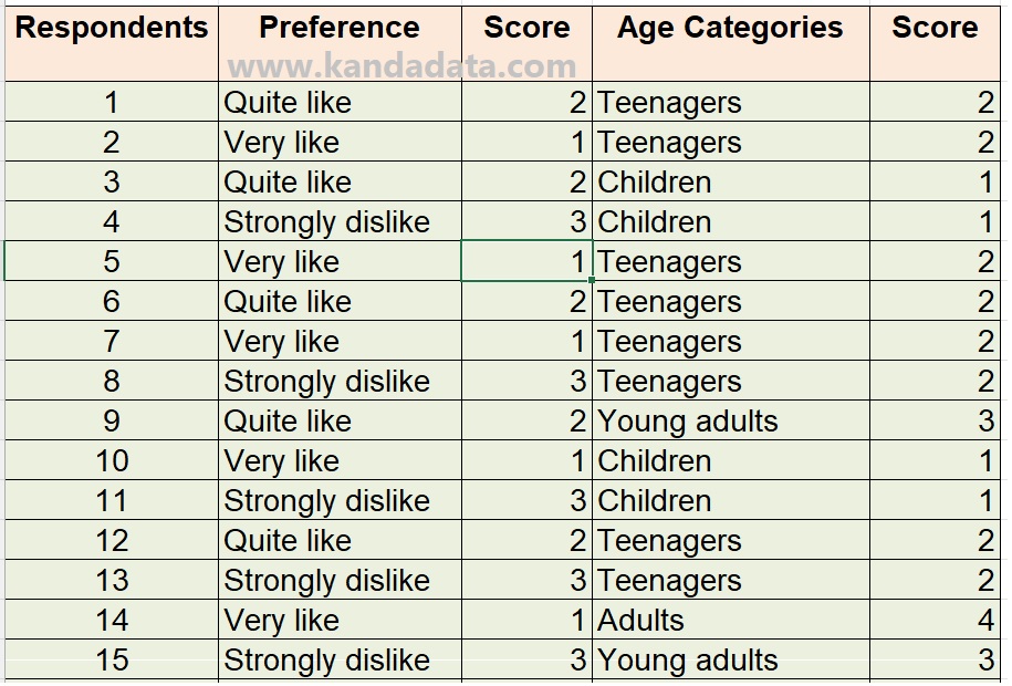
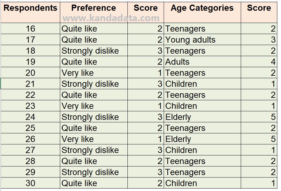
Based on the table above, the researcher converted each variable category into score form. Looking at the measurement scales of the variables, both are measured on an ordinal scale. This is because the observed categories in both variables exhibit an inherent order.
Specifically, based on the input data above, the scoring technique for each variable is as follows:
Preference:
1 = Very like
2 = Quite like
3 = Strongly dislike
Age Categories:
1 = Children
2 = Teenagers
3 = Young adults
4 = Adults
5 = Elderly
Steps for Descriptive Statistical Analysis of Non-Parametric Variables in SPSS
As a practice material for descriptive statistical analysis of non-parametric variables, we will use SPSS. As we all know, when we open the SPSS application, we encounter two windows: the data view and the variable view.
The first step researchers need to take is to set up the variables in the data view window. You can enter the variable names in the first column, which are “Preferences” and “Age.” Next, in the label column, provide more detailed information about the variable names, namely “Preferences” and “Age Categories.”
The third step is for researchers to set up the values according to the scoring technique used in the case study mentioned earlier. The preferences variable is divided into 3 scores: score 1 for “Very Like” to score 3 for “Strongly Dislike.” As for the age variable, it is divided into categories ranging from score 1 for “Children” to score 5 for “Elderly.” More detailed steps can be seen in the image below:
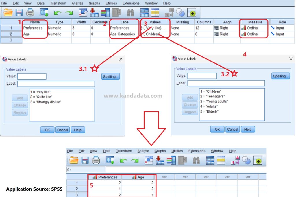
Next, after setting up the variables, we switch to the data view window in SPSS. In the data view window, we can input the data manually or copy and paste data that has been previously entered.
Previously, I have entered the data in Excel, so we can directly copy and paste the data from Excel to SPSS. After the data is properly inputted into SPSS, the next step is to perform data analysis.
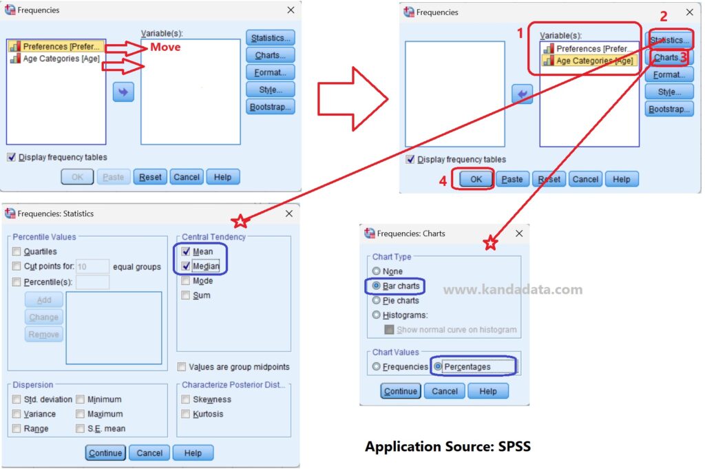
Next, click on Analyze, then select Descriptive Statistics, and click Frequencies. A Frequencies window will appear. In this window, move the Preferences variable and the Age Categories variable into the Variable(s) box.
Next, click on Statistics to display the measures of central tendency. We can view the Mean and Median values. Then, to display Charts, click on Charts. Here, I will display Bar Charts, and the values will be presented in percentages. After that, click on Continue and OK. Detailed steps of the analysis can be seen in the image below:
Interpretation of Descriptive Statistical Analysis Results
After following all the analysis steps as outlined in the tutorial written in the previous paragraph, the output will appear in SPSS, which can be seen in the image below:
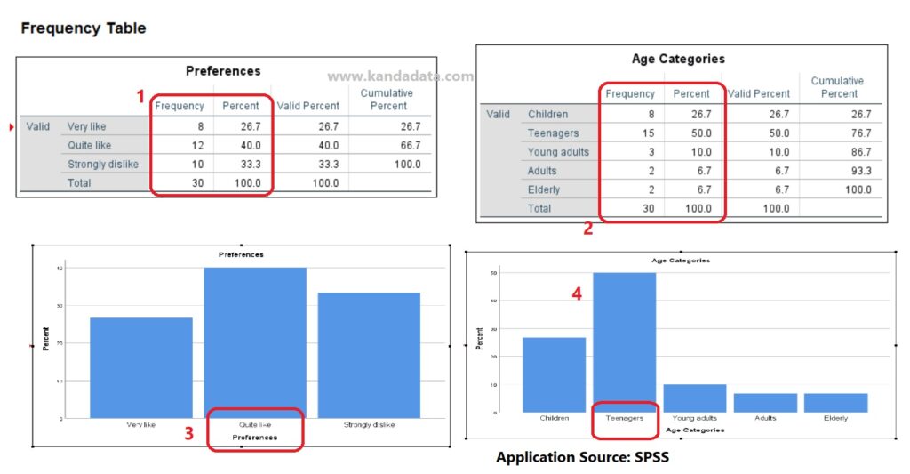
Based on the above image, I will not present the results of the measures of central tendency in this article. Instead, I will directly focus on discussing the frequency table. Based on the table above, it can be observed that the majority of consumers prefer the strawberry variant of milk.
This can be seen from 12 respondents selecting “Quite Like” and 8 respondents selecting “Very Like.” Therefore, only 33.3% of respondents dislike the strawberry-flavored pasteurized milk variant.
Furthermore, based on the image above, it can be observed that the majority of respondents are Children and Teenagers. Their combined percentage is 76.7%, with children accounting for 26.7% and teenagers accounting for 50%.
The Bar chart results also indicate that Teenagers have the highest percentage, with the highest preference for “Quite Like.” Of course, this interpretation can be further developed by the researcher to provide a more comprehensive explanation and comparison with previous research findings.
Well, this concludes the educational article that Kanda Data has written on this occasion. We hope it has been beneficial and provided new insights to those who have read the entire article. Thank you, and we hope it is useful for everyone. See you in the next educational article.
1 comment
Leave a Reply
You must be logged in to post a comment.
Pingback: Benefits of Using Cross Tabulation in Descriptive Statistical Analysis - KANDA DATA