Blog
How to Perform Linear Regression Analysis Using Excel | A Complete Step-by-Step Tutorial and Guide

In today’s post, Kanda Data provides a comprehensive tutorial on how to perform linear regression analysis using Microsoft Excel. Before we dive into the tutorial, the first step is to activate the Analysis ToolPak in Excel. Next, Kanda Data presents a case study example of research data to be analyzed using linear regression analysis.
This tutorial will guide you through the linear regression analysis steps using the Analysis Toolpak menu. A separate article will cover the tutorial on testing the assumptions required for this analysis.
How to Activate the Analysis ToolPak
Before we can use the data analysis menu in Excel, we need to ensure that the ‘Analysis ToolPak’ add-in is activated. If it’s not yet enabled, open Excel and click on File in the upper left corner.
From the several options available, then choose Options. After the Excel Options dialog box appears, select Add-ins. Then, at the bottom, ensure that ‘Excel Add-ins’ is selected in the Manage dropdown and click Go.
Finally, check the box next to Analysis ToolPak and click OK. Once these steps are completed, we can proceed to perform linear regression analysis in Excel.
How to Input Data in Excel
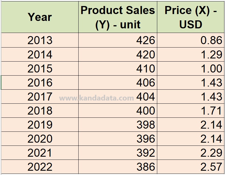
Open Excel and enter the data with the appropriate variable names. For instance, I have obtained data consisting of product sales as the dependent variable and price as the independent variable. The data we will use for practice can be seen in the table below:
How to Access the Data Analysis Menu in Excel
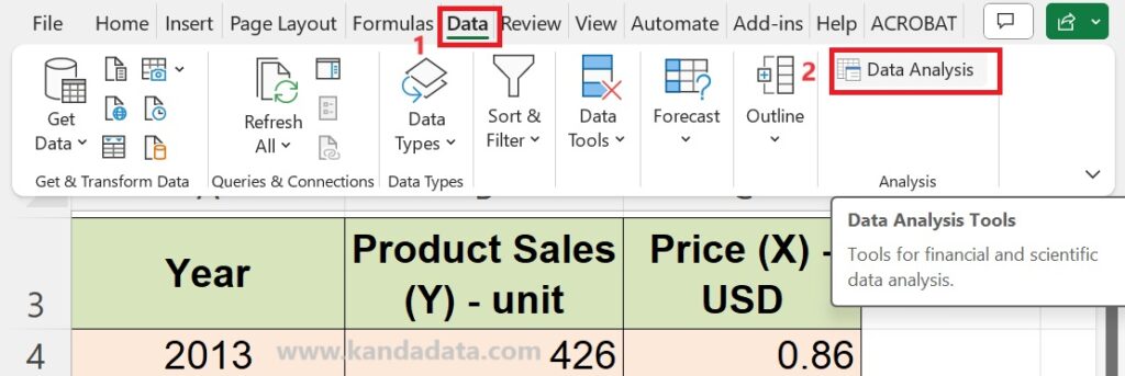
Once the Excel file is opened, then click on Data in the Ribbon, and the data analysis menu will appear as shown in the image below:
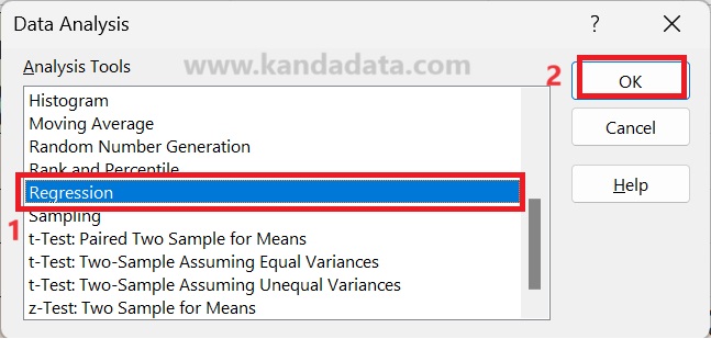
Numerous analysis options provided by Excel will then appear. Please select Regression as shown in the image below:
How to Perform Linear Regression Analysis in Excel
To input the Y variable into Excel, click the arrow as shown in the image below:
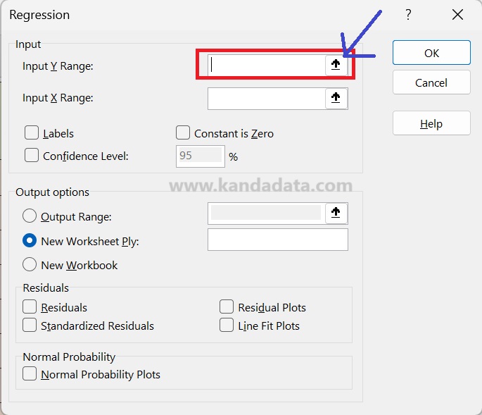
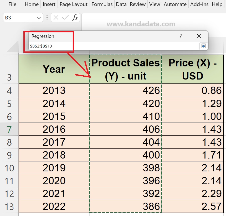
For Input Y Range:, select the data range for Your Product Sales (Y), in this case, cells B3:B13, which can be detailed as seen in the image below:
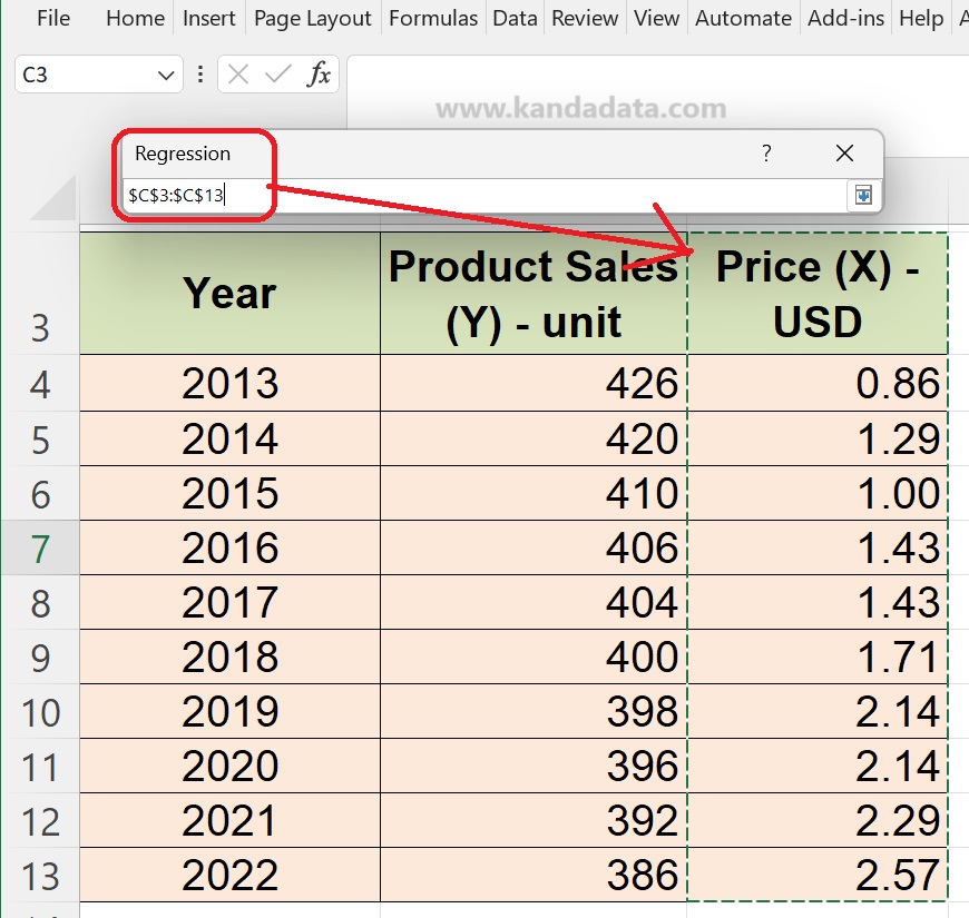
Next, for Input X Range:, select the data range for Price (X), which is cells C3:C13, as shown in the image below:
Choose the Labels option because we have column headers as variable labels, and fill in the Confidence Level with 95%. Then, choose the output location where you want the regression results to appear. I want to save the regression results in a sheet I named Output, and the steps for this can be detailed as seen in the image below:
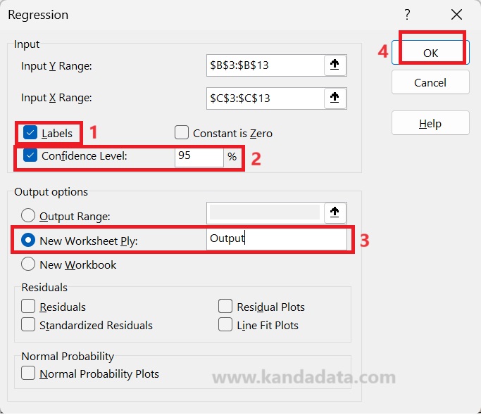
After completing these steps, then click OK. When you click OK, the output of the regression analysis results will appear, which can be detailed in the image below:

Based on the above output, we can interpret the results of the linear regression analysis. Key values to pay attention to include the coefficient of determination (R-squared), the F-statistics value in the ANOVA table, and the t-statistics for statistical hypothesis testing decisions.
Well, this is the tutorial article I can write about how to perform linear regression analysis using Excel. Hopefully, this step-by-step guide can assist those who wish to perform linear regression analysis using Excel. May it be useful and stay tuned for updates from Kanda Data next week.