Blog
Multiple Linear Regression Analysis and Interpreting the Output in Excel

We can use multiple linear regression analysis to estimate the effect of the independent variable on the dependent variable. Multiple linear regression using at least two independent variables.
Due to many researchers, lecturers, and students who use multiple linear regression analysis, I will review how to analyze and interpret the output. In a previous article, I have written an article on analyzing multiple linear regression using SPSS.
On this occasion, I will analyze multiple linear regression using excel. Excel can also help us analyze multiple linear regression quickly as we use statistical software, such as SPSS, SAS, STATA, etc.
To make it easier to understand how to analyze data and interpret it, I will give an example of a case that can be used for exercise. I use an example of a case of multiple linear regression with two independent variables.
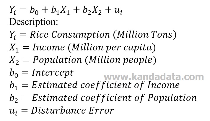
The variables I use consist of: (a) rice consumption as the dependent variable; (b) Income as the 1st independent variable; and (c) Population as the 2nd independent variable. This exercise aims to know how income and population influence rice consumption.
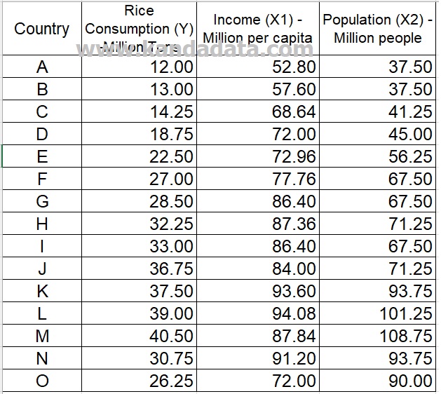
Rice consumption is measured by million tons, Income by million per capita, and population by million people. Data were analyzed using the results of variable observations in 15 countries. The specifications for multiple linear regression equations can be arranged as follows:
Data Input
The next stage after the specification of the regression equation is to input data. Data can be directly inputted into excel.
Next, you can create 4 columns which are then filled with the name of the country and the name of the variable (1 dependent variable and 2 independent variables). Furthermore, the row is filled with data from each observation result. The data used for the exercise can be seen in the table below:
Data Analysis Tools in Excel
In several previous articles, I have written about tutorials on calculating simple linear regression and multiple linear regression manually using excel. But this time, I will use the data analysis tools provided in excel.
Data analysis tools in excel can be seen in the “Data” menu, and then you will find “Data Analysis” in the upper right corner of your excel. If you don’t find the thing in question, you need to activate the toolpak first in excel.
To enable “Data Analysis” in excel, you can follow the tutorial I wrote in the article entitled: “How to Activate and Load the Data Analysis Toolpak in Excel.”
How to Analyze Multiple Linear Regression in Excel
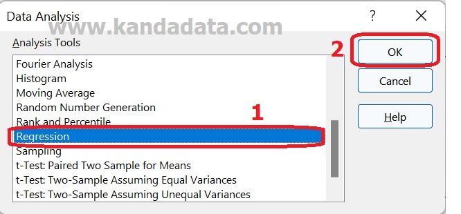
To perform multiple linear regression analysis using excel, you click “Data” and “Data Analysis” in the upper right corner.
The “Data Analysis” window will then appear, then you select regression as shown below:
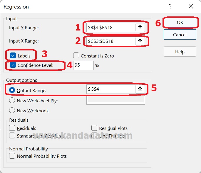
The next step is to input the variable label and all dependent variable data into the “Input Y Range:” box. You then input the variable label and independent variable data into the “Input X Range:” box.
How do input label variables and data?; you can block all the labels and data in the excel sheet. Next, you activate “Labels” and “Confidence Level” For the Confidence level, I choose a p-value of 5% (0.05).
There are 3 options for storing the analysis output: the same sheet, creating a new sheet, and a new workbook. I chose to display it on the same sheet.
You can also generate residual values and normal probability plots (optional). Then you click OK to bring up the output of the analysis. The stages in detail can be seen in the image below:
Multiple Linear Regression Analysis Output Interpretation
The output displayed in excel is divided into three tables, namely summary output, ANOVA, and coefficient table. The resulting output summary table is as shown below:
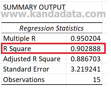
There is 5 information displayed in the summary output, namely Multiple R, R Square, Adjusted R Square, standard error, and observations. From this information, R Square and Adjusted R Square can be used to estimate the model’s goodness.
The value of R Square can be seen that the value is 0.902888. You can interpret that the variation of the rice consumption variable of 90.29% can be explained by the variation of the income and population variables. The remaining 9.71% is explained by other variables not included in the equation model.
Next, we move to the 2nd table, namely the ANOVA table. The ANOVA table can be used to test the research hypothesis. For example, I formulate a research hypothesis as follows:
Ho: Income and Population simultaneously have no significant effect on rice consumption
H1: Simultaneous Income and population have a significant effect on rice consumption
We can see from the F value in the ANOVA table to test this hypothesis. The ANOVA table from the results of multiple linear regression analysis can be seen in the image below:
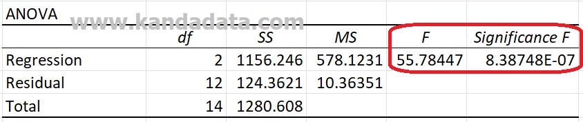
To test the hypothesis, we can use 2 criteria: (1) comparing the F value with the F table and (2) looking at the P-value. If you use the 1st criterion, you have to find the F value in the table first.
Here I will use the second criterion, namely by looking at the P-Value. The p-value in excel is displayed with the label “Significance F” The written significance value of F is 8.38748E-07, which means the same as that the P-value is less than 5% (P<0.05).
Thus we can conclude that Ho is rejected. Since Ho is rejected, we accept the alternative hypothesis (H1 is accepted). Therefore, we can conclude that Income and Population simultaneously have a significant effect on rice consumption.
The last table on the output of multiple linear regression in excel is the coefficient table. This table can be used to test the research hypothesis partially. For example, I formulate a research hypothesis as follows:
Ho: Income partially has no significant effect on rice consumption
H1: Income partially has a significant effect on rice consumption
Ho: Population partially has no significant effect on rice consumption
H1: Population partially has a significant effect on rice consumption
Two criteria can be used to test the hypothesis: (1) comparing the t-stat value with the t-table and (2) looking at the P-value. Using the 1st criterion, you must first find the t Table’s value.
The coefficient table from the results of multiple linear regression analysis can be seen in the image below:
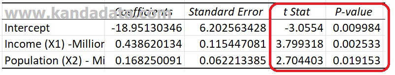
Here I will use the second criterion, namely by looking at the P-Value value. The p-value in excel is displayed with the label “P-value” The P-value for the income variable is 0.002533, meaning that the P-value is smaller than 5% (P<0.05).
Thus, the null hypothesis is rejected (accepted alternative hypothesis). Therefore, it can be concluded that Income partially has a significant effect on rice consumption.
Furthermore, the P-value for the population variable is 0.019153, meaning that the P-value is smaller than 5% (P<0.05). Thus, the null hypothesis is rejected (accepted alternative hypothesis). Therefore, it can be concluded that Population partially has a significant effect on rice consumption. To enhance your understanding of multiple linear regression analysis and how to interpret the output effectively, I recommend the book Regression Modeling Strategies: With Applications to Linear Models, Logistic and Ordinal Regression, and Survival Analysis.
Well, I hope this article will be beneficial for all of us. Please feel free to write it down in the comments below if there is a question. See you in the next article!