Blog
How to Analyze and Interpret the Durbin-Watson Test for Autocorrelation

Researchers can use regression analysis to determine the effect of independent variables on the dependent variable. The data used in the regression analysis can use cross-section, time series, and panel data. On this occasion, Kanda Data will discuss regression analysis using time series data.
The regression estimation coefficient using time-series data must meet several assumption requirements to obtain the best linear unbiased estimator. One of the assumption tests required for conducting is the autocorrelation test. The autocorrelation test was carried out to test the residual correlation in the t period with the previous period (t-1).
The linear regression model, where the residuals in period t correlate with the previous period, indicates that the residuals are not independent of one observation to another. Autocorrelation can be detected using several tests, for example, run tests, Durbin Watson tests, and Breusch-Godfrey tests. On this occasion, I will provide a tutorial on analyzing and interpreting the Durbin-Watson test for autocorrelation.
The Durbin-Watson test can use several data processing tools, one of which is SPSS. I will provide step by step regarding the stages of the Durbin-Watson test using SPSS. To make it easier to understand this tutorial, I have prepared exercise materials for data analysis. You can also use the time series data you have following the tutorial I will write on this occasion.
Mini-research case study
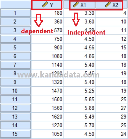
An example of a mini-research used as exercise material on this occasion is multiple linear regression with two independent variables. The data used in this study used 15 months of monthly time series data. This study aims to investigate the effect of advertising costs and marketing staff on product sales.
Based on the specifications of the equation compiled by the researcher, product sales are used as the dependent variable, while advertising costs and marketing staff are used as independent variables. The data measurement scale of the variables used in this study uses a ratio scale. The results of the time series data collection in detail can be seen in the table below:
How to analyze the Durbin-Watson test
The Durbin-Watson test can be used in several ways: statistical tools or manual calculations. I will provide a tutorial on how to analyze using SPSS.
Based on the data the researcher has collected can be input directly into the data view in SPSS. Another alternative is that researchers can also input data into Excel and copy and paste it into SPSS. Furthermore, in the view variable in SPSS, the researcher needs to fill in the variables’ specifications, including variable names, labels, and data measurement scales.
After the researcher inputs all the data that has been collected into SPSS, to obtain the Durbin Watson value, the researcher only needs to do a few steps in SPSS. In detail, the stages of the analysis start from analyze > regression > linear.
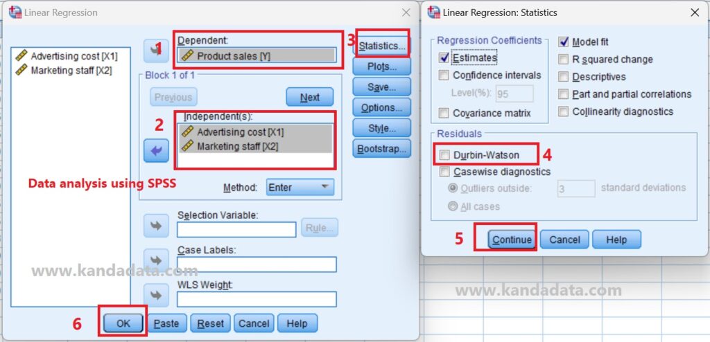
Then a linear regression window will appear, and the researcher needs to move the product sales variable into the dependent box. Furthermore, the variable costs of advertising and marketing staff are transferred to the independent box.
The researcher needs to click on the statistic to obtain the Durbin-Watson value. After clicking on statistics, two sections of analysis options will appear, including regression coefficients and residuals. In the residual section, you must activate Durbin-Watson, click continue, and click ok. The detailed stages of the Durbin Watson analysis using SPSS can be seen in the image below:
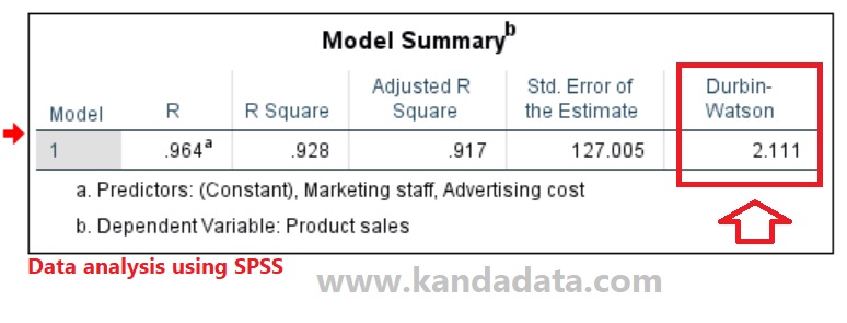
After the researcher completed all the stages in the Durbin-Watson test, there were several outputs that SPSS displayed. There were several components in the SPSS output, including a model summary, ANOVA, and estimated coefficients at the SPSS output.
Durbin-Watson values can be found in the model summary. Based on the Durbin-Watson test using SPSS, a value of 2.111 was obtained. In detail, the output of the Durbin-Watson test for autocorrelation using SPSS can be seen in the image below:
How to interpret the Durbin-Watson test
The next step that needs to be understood by researchers is how to draw conclusions based on the value of the Durbin-Watson test. The Durbin-Watson test can be compared with the Lower Durbin (dL) and Upper Durbin (dU) values.
To obtain dL and dU values, researchers can use Durbin-Watson tables. I use the Durbin Watson table with an Alpha of 5% in this tutorial. In the Durbin-Watson table, the column section includes the number of independent variables used in the study. The number of independent variables is denoted by k.
Furthermore, the row contains the number of observations used in the study. To make it easier to understand how to read the Durbin-Watson table, you can see the Durbin Watson table below:

Based on the research example using multiple linear regression with two independent variables, it shows that the value of k = 2. Furthermore, with the number of observations of 15 and k = 2, the dL value is 0.9455, and the dU value is 1.5432.
Based on these values, the researcher needs to calculate the 4-dU and 4-dL values to draw conclusions. In detail, these values can be seen in the image below:
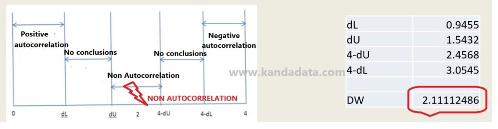
Based on the picture above, it can be seen that there are several parts. Conclude options consist of positive autocorrelation, no conclusion, non-autocorrelation, and negative autocorrelation. The researcher needs to input the values of dL, dU, 4-dL, and 4-dU, respectively.
Based on the picture above, the Durbin-Watson value for the SPSS output is 2.111. The Durbin-Watson test value is between the dU and 4-dL values. Because the value of the Durbin-Watson test is between dU and 4-dL, it can be concluded that the regression equation tested in the mini-study example does not show autocorrelation.
What should I do if autocorrelation occurs?
The results of the Durbin-Watson test show that the regression equation does not show autocorrelation. Thus, researchers can examine and investigate other test requirements. It is intended so that the estimated coefficients are not biased and we can obtain the best linear unbiased estimator.
Then the question is, what if it turns out that there is autocorrelation? For example, the test results showed positive autocorrelation or negative autocorrelation. If there is an autocorrelation, the researcher needs to solve the autocorrelation.
How to solve autocorrelation
There are several ways that researchers can do to solve autocorrelation. The first step that can be done is that researchers can consider adding new data. The fewer samples taken in the study will potentially increase the existence of problems in the assumption test.
Another alternative step that can be taken is to consider entering the lag variable from the dependent variable into an independent variable. In addition, researchers can also remove one variable with a high correlation.
To gain a deeper understanding of autocorrelation and other essential concepts in time series data, I recommend the book Time Series Analysis, 1st Edition. This comprehensive guide covers key teheoy and methods.
Another alternative researchers can consider is using the variable transformation method. Re-analysis of the entire model using the values of the transformed variables can be used to solve autocorrelation. That’s all I can write about How to Analyze and Interpret the Durbin-Watson Test for Autocorrelation on this occasion. Hopefully, this article will be helpful for all of you. Thank you!