Blog
How to Test for Normality in Linear Regression Analysis Using R Studio

Testing for normality in linear regression analysis is a crucial part of inferential method assumptions, requiring regression residuals to be normally distributed. Residuals are the differences between observed values and those predicted by the linear regression model.
It’s vital to perform a normality test to ensure that the residuals in the regression equation are normally distributed. The most commonly used tests for regression normality among researchers are the Shapiro-Wilk test and the Kolmogorov-Smirnov test.
The assumption of normality in residuals is important as it can affect the validity of the model’s estimation results, as well as the consistency and accuracy of the model’s regression predictions. If the distribution of residuals is not normal, the results of the regression analysis may be biased.
If residuals are not normally distributed, researchers can consider several alternatives, such as increasing the data size, modifying the equation specifications, data transformation, and other methods. In R Studio, normality testing can be conducted using various statistical methods and functions.
One common method for testing normality in R Studio is the Shapiro-Wilk test. Besides this, R Studio also offers various other normality tests, such as the Kolmogorov-Smirnov test, Lilliefors test, and Anderson-Darling test.
These tests yield a p-value, which helps decide whether the residual distribution can be considered normal. A p-value greater than a predetermined significance level (e.g., alpha 0.05) indicates insufficient evidence to reject the null hypothesis (accepting the alternative hypothesis), suggesting that the residuals are normally distributed.
Importing Data from Excel to R Studio
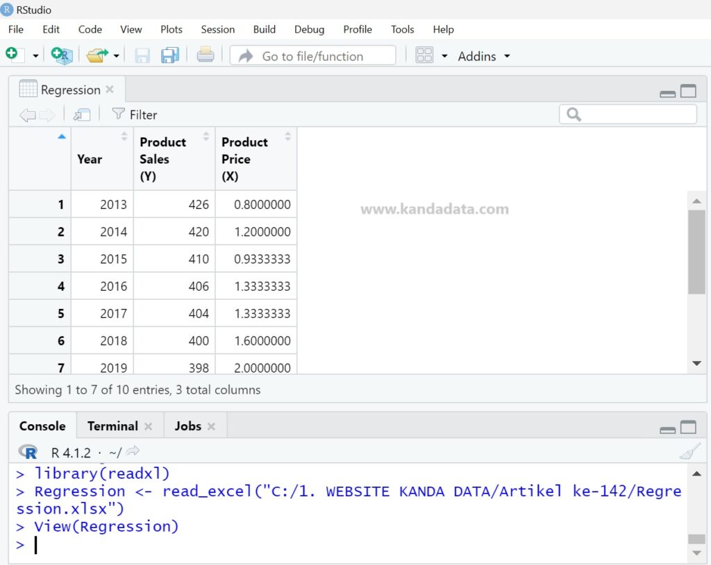
In R Studio, data import from Excel can be done in several ways. The most common method involves using the ‘readxl’ and ‘openxlsx’ commands. To import data from an Excel file in R Studio, you would write:
> library(readxl)
> Regression <- read_excel(“C:/KANDA DATA/Regression.xlsx”)
> View(Regression)
Adjust the file path and Excel file name as per your requirements. Following this tutorial, the imported data will appear in R Studio as shown:
Normality Test in Regression Analysis Using Residuals
Residuals are the differences between observed values and those predicted by the model. In simple linear regression, residuals are calculated by subtracting the observed value from the predicted value. Mathematically, a residual (e) is represented as e = y – ŷ, where y is the actual observed value, and ŷ is the value predicted by the regression model. Residuals are used to evaluate the quality of a model, with smaller residuals indicating a model accurately predicts data.
In regression normality testing, the focus is on the values of the residuals. Therefore, it’s important for researchers to calculate the residuals in linear regression analysis. To find the residual values, first write the following command:
model <- lm(Y ~ X, data = Regression)
In the above command, replace Y and X with the labels of the variables in your R Studio. ‘Regression’ is the name of the Excel file I used. Next, to display the residual values, write:
residuals_model <- residuals(model)
Once you’ve entered the above command, the residuals are ready for normality testing. You can choose any one of the normality tests for linear regression analysis.
Testing for Normality in R Studio
For normality testing using R Studio, here I provide a tutorial using the Shapiro-Wilk and Kolmogorov-Smirnov Tests. For the Shapiro-Wilk test in regression analysis, please write the following command:
shapiro.test(residuals_model)
Next, for the Kolmogorov-Smirnov test, you can write the following command in R Studio:
ks.test(residuals_model, “pnorm”)
Based on the detailed results of the Shapiro-Wilk and Kolmogorov-Smirnov tests using R Studio, the findings are as follows:
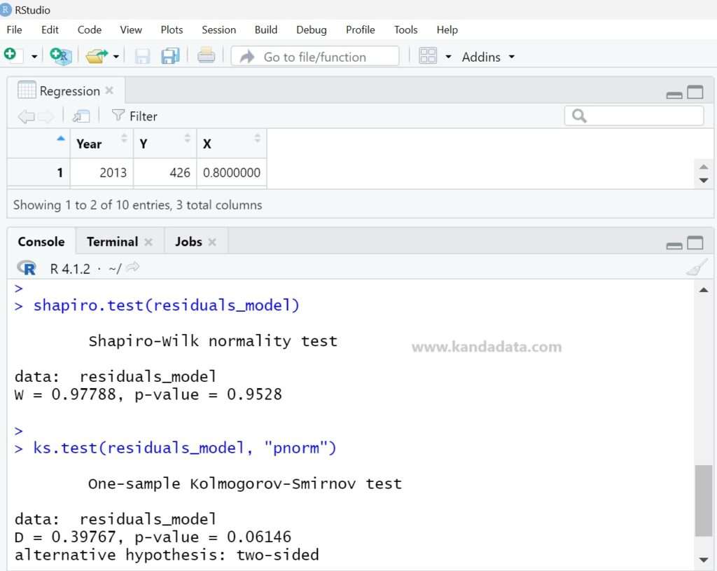
The p-value from the normality test can help determine the extent to which the residual distribution approximates a normal distribution. A p-value > 0.05 indicates that there is not enough evidence to reject the null hypothesis, meaning the residual distribution can be considered normal.
Well, this is the article that I can write at this opportunity. Hopefully, it is beneficial and adds new knowledge value for those in need. Stay tuned for updates from Kanda Data next week. Thank you.