Blog
How to Test Normality of Residuals in Linear Regression and Interpretation in R (Part 4)

The normality test of residuals is one of the assumptions required in the multiple linear regression analysis using the ordinary least square (OLS) method. The normality test of residuals is aimed to ensure that the residuals are normally distributed.
Residuals in linear regression analysis are obtained by subtracting the actual dependent variable values from the predicted dependent variable values (actual Y minus predicted Y). The predicted values of the dependent variable can be obtained after estimating the linear regression coefficients.
A detailed tutorial on how to obtain residual values can be found in the previous article titled: “How to Find Residual Value in Multiple Linear Regression using Excel” and other articles such as “Create Residual and Y Predicted in Excel“.
The expected result of the normality test in linear regression is that the residuals are normally distributed. Therefore, researchers need to perform a normality test of residuals in the regression equation to ensure that the residuals are normally distributed.
For researchers analyzing data, both cross-sectional and time-series data, using the OLS method, it is necessary to test the normality assumption of residuals.
There are several methods of testing to determine whether residuals are normally distributed or not, one of which is the Shapiro-Wilk test using R Studio. This is part 4 of the tutorial that discusses how to test the normality of residuals and how to interpret the results in R.
Formulating the hypothesis of normality test of residuals
To test whether the residuals are normally distributed or not, researchers can formulate a statistical hypothesis. The statistical hypothesis can be formulated in the null hypothesis and the alternative hypothesis.
The statistical hypothesis and the acceptance criteria for the normality test of residuals in R can be formulated as follows:
Ho: p-value >0.05 = Residuals are normally distributed
Ha: p-value <0.05 = Residuals are not normally distributed
Sample data for normality test of residuals
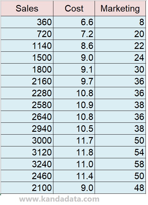
As a practice exercise for testing normality of residuals, a multiple linear regression sample data has been prepared here. The aim of the study is to determine the influence of cost and marketing on sales.
Therefore, cost and marketing are used as independent variables and sales are used as the dependent variable. The data collected by the researcher in detail can be seen in the table below:
Importing Data from Excel to R Application for Normality Test of Residuals
To import data in R, the researcher can click on File and then select Import dataset from the various options available. Since the data was saved in Excel, select “from Excel”.
The next step is to browse and locate the Excel file, and then a preview of the data input in Excel will appear. Click on import to complete the process. If these steps are followed systematically, the preview of the imported data from Excel will appear in R studio.
Syntax for Normality Test of Residuals in R
To conduct a normality test of residuals in R, the researcher needs to perform multiple linear regression analysis first by typing the syntax “Sales ~ Cost + Marketing” and adjusting the number of variables used. The labels of the variables should be typed exactly as shown in the preview in R studio, including capital and small letters.
Next, the syntax “data = Multiple_Linear_Regression” indicates the data source used, and it should be written exactly as the file name used when importing data.
After pressing enter, the next step is to type “shapiro.test(resid(model))”. This syntax is used to show the results of the Shapiro-Wilk test. The detailed syntax of the normality test of residuals using Shapiro-Wilk can be seen in the figure below:

Interpretation of Residual Normality Test Output in R
The output of the normality test of residuals using Shapiro-Wilk in R is similar to other analysis tools. The detailed output of the Shapiro-Wilk test in R can be seen in the figure below:
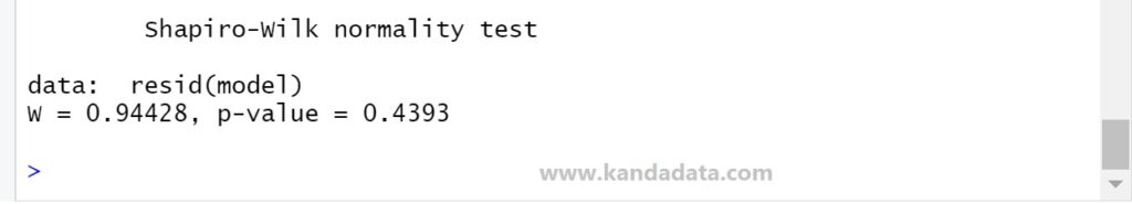
Based on the figure above, it is known that the Shapiro-Wilk value (W) is 0.94428. The p-value is 0.4393. Furthermore, the statistical hypothesis testing criteria using the acceptance criteria are as follows:
Ho: p-value > 0.05 = Residuals are normally distributed
Ha: p-value < 0.05 = Residuals are not normally distributed
Based on the acceptance criteria, the p-value is greater than 0.05, so the null hypothesis is accepted. Since the null hypothesis is accepted, it can be concluded that the residuals are normally distributed.
Therefore, the regression equation satisfies one of the assumptions of the OLS linear regression method, which is normal distribution of residuals. This test result shows that the regression model meets the normality assumption. This is the end of part 4 of this article. Stay tuned for the next part.